I had an email from Bobcat today asking how to lookup data that is spread across multiple columns.
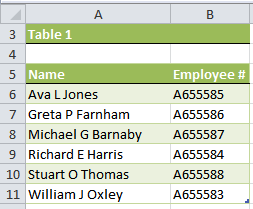
Table 1 has data with the name in just one column:
And Table 2 has the name across 3 columns (D, E and F):
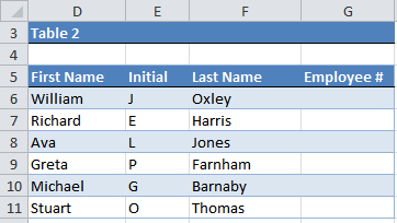
We want to find the Employee number from Table 1 and put it in column G of Table 2.
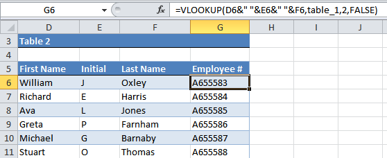
The solution is quite simple. We just need to join together the cells containing the name in Table 2, before looking them up in Table 1.
We can do this within a VLOOKUP formula like this:
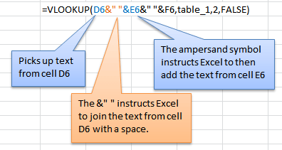
=VLOOKUP(D6&" "&E6&" "&F6,table_1,2,FALSE)
Note: table_1 in the above formula is the named range for cells A6:B11
See in the formula bar how I’ve joined the text from columns D, E and F together using the ampersand symbol. I’ve also added a space between the text by inserting double quotes with a space between.
The VLOOKUP formula is resolving the D6&" "&E6&" "&F6 arguments of the formula like this:
=VLOOKUP(William J Oxley,table_1,2,FALSE)
Thanks for your question Bobcat.

I want to invest 30000 per annum for 10 years at 10% per annum but want to allow the value invested of 30000 annually to be depreciated by 9% per annum to allow for currency inflation and provide a realistic value result
if there is anything that can help me to find 6 values with target sum out 150 or more values???
Hi Mommar,
If you have 1000 values, there are 1368173298991500 possible combinations of 6 values:=COMBIN(1000,6)
You will need a user defined function to build all possible combinations, and list those where their sum is above 150. You will need a powerful computer to do those calculations, a regular computer might take a while to process that.
i want to know allot about excel..
Hi,
Hopefully we can help you out. Just browse though our blog, there’s plenty to learn there. Or take one of our Excel courses.
Regards
Phil
NO THIS FORMULA NOT WORK WHEN TABLE_2 NOT ARRANGED LIKE TABLE_1
WE SHALL HAVE TO USE VLOOKUP WITH CHOOSE IN ARRAY FORMULA
Not necessarily. INDEX & MATCH can handle lookups where the order of columns is not suitable for VLOOKUP. I would only use an array formula as a last resort.
Mynda
I have a similar situation I have one table that is in a file named Shelby Name ID.xlsx , it has 2 columns. Column A has the first and last name in it and Column 2 is an ID
I have another Table in a file named IndividualExport.csv , it has numerous columns with the first name, middle name, and last name in columns H,I and J respectfully. The first column of this Table is labeled LInk ID.
I am trying to put the Link ID number from the IndividualExport.csv to the 3rd column in the Shelby Name ID.xlsx
When I try your formula I keep getting #VALUE!. I am familiar with the vlookup function but not with tables so I think I am writing the formula wrong. Here is the formula I am using and it is in the 3rd column of the Shelby Name ID file;
=VLOOKUP([@Name],IndividualExport.csv!Table1[@First]&” “&IndividualExport.csv!Table1[@Middle]&” “&IndividualExport.csv!Table1[@Last],1,FALSE)
Hi Mike,
As you already know, VLOOKUP function has 4 arguments:
-lookup_value, table_array, col_index_num, and range_lookup.
In this article, the name is concatenated into the lookup_value argument, then the function is searching a match for the resulting string in table_array argument. In your formula, you are concatenating 3 columns of data into the table_array argument, which is totally different from concatenating 3 cells, as the tables do have multiple rows. The formula turns into an array formula, which needs to be entered as an array formula, with CSE (Ctrl+Shift+Enter), not just Enter after editing the formula. If the correct combination of keys is entered (Ctrl+Shift+Enter), then you will see that in the formula bar, the formula is wrapped into a set of curly brackets: { }
These should not be entered manually, they are automatically introduced when CSE is pressed, and they represent array formulas.
Cheers,
Catalin
I am trying to lookup a column from a different tab, but it has to match two different criteria in order to return the correct value. For example, I have item “1” going to “A” and “B” at two different prices. The two different tabs are not formatted the same way, but they both have the same information to return the correct value if I could just figure out the formula.
Thanks.
Hi Anthony,
You can upload a sample workbook with your calculations on our Help Desk system, i will gladly help you if you provide clear details.
Catalin
Will I be charged for going through the help desk?
Of course not, you’re safe there 🙂
Catalin, It worked, Thank You very much.
Please if you can help me with this, Suppose A4 is $100, B4 is $40, C4 is $50, F4 is $25. G4 is$20. I need to have 5% of the lower of B4 and G4 in column D4.
Hi Hemant,
MIN function (MAX also) allows you to refer up to 255 numbers or ranges, like:
=MIN(B4:C4,E4:G4)*0.05
Catalin
Catalin, Thank You very much for all your help.
You’re wellcome Hemant 🙂
Hi Mynda,
Suppose A4 is $100, B4 is $40. I need to have 5% of the lower of two cells in C4. How should I write it in excel formula. Thank You for your help.
Hi Hemant,
Use: =Min(A4:B4)*0.05
Catalin
Great Advice! Thank you!
I have a Question tho, how must the Formula be entered if Table 1’s A-Column was actually 3 Columns, just like in Table 2? Meaning you’d still compare the 3 Columns but Source Table as well as Entry Table are the same Amount of Columns with the 4th (G) being the one that Data is to be populated in.
20 to 30 column and all column contain some value and all column which contain some value then total of all column and which columns total are lowest then lowest column value in another 31 column shows
Hi,
Can you upload a sample workbook, with detailed description of what are you trying to achieve? It will be easier for us to understand the situation, and the solution will come faster!:) You can use the Help Desk: https://www.myonlinetraininghub.com/helpdesk/
Best,
Catalin
nice and thanks
You’re welcome, Kashif 🙂
Hi,
I have a problem with a vlookup at the moment – how do i contact you for help
Regards
Tim
Hi Tim,
Please explain your concerns here: HELP DESK.
It would be best if you can send a mock file.
Cheers,
CarloE
What if we wanted to match three fields of data in on the look up sheet?
If the three fields match 3 fields in the look up sheet true = one of the fields and false = “”
Hi Bill,
I wrote another tutorial on looking up multiple values and matching them to multiple columns here.
In it I show you a way you can use VLOOKUP and the IF function to do this, but at the bottom of the tutorial I show you another (better) way with INDEX and MATCH. Given your question it would go a bit like this:
I hope that helps. If you get stuck please send me your workbook with specific instructions on what you want and where via the help desk.
Kind regards,
Mynda.
Hi
I would like to create a vlookup that would look in a specifica column all the word attached without space and insert one..do you think will be possible?
Many thanks
Hi Caterina,
VLOOKUP is not the function for the job. You have a few options depending on your data.
Does your data have a character where you want the space e.g. a hypen, comma, full stop etc.?
If so you could just use the Find & Replace tool:
1. Select the cells containing the data you want your spaces added to.
2. CTRL+H to open Find & Replace tool
3. Type in the character you want to replace in the ‘Find’ field
4. Enter a space in the ‘Replace’ field
5. Click Replace or Replace All
If that doesn’t/won’t work please send me your workbook via the help desk so I can see what you’re working with and give you a specific solution.
Kind regards,
Mynda.
hi,
linda i want a mltipal name and a diffrent heads i want if i enter head name the other branches of a head is auto,
Hi Adnan,
I’m sorry I don’t understand your question. Can you please send me your Excel file with your data and specific requirements so I can better understand your question.
Thanks,
Mynda.
Can we do the reverse? I’m importing into a document where the concatenate is placed but I cannot place the concat in the document the data is coming from. In my instance, Doc 1 has site-driver-descri (site, driver, first 5 characters of description) all in col B
The array would be from Doc 2 with no concatenate. Doc 2 has Col A for “site”, Col B for “driver” and i need the first 5 characters of the descrip housed in Col C to match. I need to pull in the value from Doc 2, column J.
A concatenate array seems doable, but I cannot ifgure it out. I attempted to use “Lookup” solution but retrieved no results with that.
Hi Abby,
I was having a hard time really trying to work around formulas.
So instead of going empty handed on this one, I am giving you a VBA customized function.
Here’s the deal:
1) ALT + F11 ( this will bring you to the VBE Window)
2) In the VBE Window, Go To INSERT menu, Add MODULE (NOTE: NOT CLASS MODULE)
3) In the Module, Paste this code
Function MyVLookup(LookUpValue As String, TBLArray As Range, Col_Return As Integer) As String
    Dim r As Long
    For r = TBLArray.Cells(1, 1).Row To TBLArray.Rows.count
        If TBLArray.Cells(r, 1) & TBLArray.Cells(r, 2) & TBLArray.Cells(r, 3) Like LookUpValue & "*" Then
            MyVLookup = TBLArray(r, Col_Return).Value
            Exit Function
        Else
        End If
    Next
End Function
4 Here’s how the formula is used- just like any Excel Function
MyVlookup(LookupValue,TBLArray, Col_to_Return)
REMINDERS:
1 You might encounter security warnings. Just trust it.
2 If VBA is not working, just go to Excel Options, Trust Center, Trust Center Settings, Enable Macro and ActiveX
Cheers.
CarloE
PS: This is so tailor-made for you that I save ourselves the hassle of creating a very dynamic one. In short,
The Values that this function will look for will be in Cols:A, B, and C only.
Now you may change 1(A), 2 (B)or 3 (C) in the function–shown below in italics– if you want to have another columns to be looked up or you can copy the function in the same module and name it MyVLOOKUP2 etc., and play with the columns you like to be looked up. You may also delete or add more columns by deleting the part “TBLArray.Cells(r,1)” or adding more, respectively.
Would this work to find the corresponding text value in column “x” when my lookup might be in one of 3 columns
Eg. I have a product available to order from 3 different companies – each company has a different item code. I want to type in the code from any company and find the product name in column “x”
Tx
Hi Kate,
You can use this array formula:
Entered with CTRL+SHIFT+ENTER as this is an array formula.
Where your 3 companies item codes are in cells A2:C6, your product name is in cells D2:D6, row 1 contains your headings and cell F1 contains the product code you want to lookup. If your data starts further down the worksheet than row 2 then you will need to change the -1 in the *ROW($A$2:$C$6)-1 part of the formula accordingly. i.e. I have taken -1 off the ROW formula to account for the header row in row 1, but if your data starts in say row 4 then you would have ROW($A$2:$C$6)-3.
I hope that helps.
Mynda
How about in the opposite situation?
I have around 8,000 cell values displayed in the same format:
1 019784 FILTER BAG FRAME
21 090016 INSEAL 15mmx1.5mm 90mm LONG
I need the “1” (acts as an identification point for a position in the photo diagram) to be extracted into a separate cell, the “019784” (order code) to be extracted into another separate cell and “FILTER BAG FRAME” (product description) to be extracted in another separate cell for all 9,000 cells.
N.B.
-The identification point or position number can be either 1 or 2 digits but is always delimited by a space only after the numeric value of 1 or 2 digits.
-The order code varies in it’s character count but there is a space before an after the order code value
-The description has spaces throughout the sentence as per above example and there are sometimes numeric values in the description
Can you help me with a formula to split the one cell into 3?
Hi Michael,
You can use the MID and FIND functions for this:
To extract the order code:
=MID(A1,FIND(" ",A1)+1,SEARCH(" ",A1,4)-SEARCH(" ",A1)-1)To extract the product description:
=MID(A1,FIND(" ",A1,4)+1,99)Kind regards,
Mynda.
I need the excel of the above explanation
Hi Tanveer,
I don’t know what you mean. Can you please explain in a different way?
Kind regards,
Mynda.
What if Table 1 also contains the First Name, Initial and Last Name in separate columns? There is no way to show anything like that in the array. I have solved that by adding a new column and joining them in the new column but is there a way to do it by another way? Like using if or something else nested?
Hi Ali,
You can use the LOOKUP function like this:
Where columns G, H and I contain the values you want to lookup and A,B and C contain the table you’re looking up with the result you want returned in column D.
Thanks to Roberto for suggesting that solution.
I hope that helps.
Mynda.
Mynda,
I keep getting the #Value! error code on this formula. I had the exact same Question as Ali.
I tried the formula and also variation with ,4) or ,4,FALSE) added to the end of your formula but nothing works.
Here: =LOOKUP(F21&G21&H21,Sheet1!$A$2:$A$350&$B$2:$B$350&$C$2:$C$350&$D$2:$D$350)
Data Jan 2010 – Dec 2010 is the Entry Sheet Column F (City),G (county) & H (State) will be entered and D (Zip) needs to be populated with help of the Index Sheet 1 (Library so to speak).
Index Data is in Sheet 1 Column A-D (City, County, State & Zip)
So IF F&G&H match A&B&C of Sheet 1 then copy Column D data into Data Sheet.
Could you help me please?
Thank you!
Diana
Mynda,
disregard my previous Question! I got it! 🙂 Here: =LOOKUP(F21&G21&H21,Sheet1!$A$2:$A$350&$B$2:$B$350&$C$2:$C$350&$D$2:$D$350,Sheet1!D2:D350)
Glad you figured it out, Diana 🙂
What if data is not separated in different columns? Criteria are on the first row and the first column, just like this one:
A B C D E
1 0.1 0.2 0.3 0.4 0.5
2 0.6 0.7 0.8 0.9 1.0
3 1.1 1.2 1.3 1.4 1.5
What is the formula for returning “1.1” if “A” and “3” are given?
Thank you!
Hi Nicole,
I’m not understanding your question 100% but if you only want to look up the values in one column then you can use a regular VLOOKUP formula.
If that’s not what you meant, please let me know.
Kind regards,
Mynda.
Im like both V&HLOOKUP, but my usually, commece is VLOOKUP. I am trying to looking for VLOOKUP within multiple criteria. And once again I seeking for advice to to work Piviot excel table
Hi Kosal,
I’m sorry I don’t understand what you’re having trouble with. Can you please email me with a specific example.
Thanks,
Mynda.