Toggle Top N with Slicers

Power Pivot course member, Peter, asked if it was possible to toggle the top n with a Slicer for a Pivot Chart and the answer is yes! With Power Pivot and disconnected tables, we can create interactive charts like this:

Watch the Video

Download Workbook

Setup Power Pivot Toggle Top N with Slicers

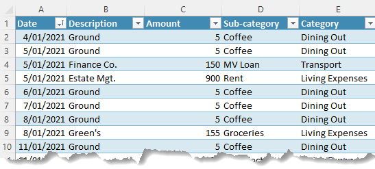
I’m using some sample data stored in an Excel Table called ‘Data’. You can see below it is grouped by category and sub-category and I want to filter the top n sub-categories:

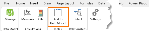
We start by loading the data into Power Pivot, preferably via Power Query. Alternatively, if your data is in an Excel Table you can use the ‘Add to Data Model’ button on the Power Pivot tab:

I also need to load a table that stores the top n values I want the user to be able to select in the Slicer into Power Pivot. You can see in the image below the table is called TopN:

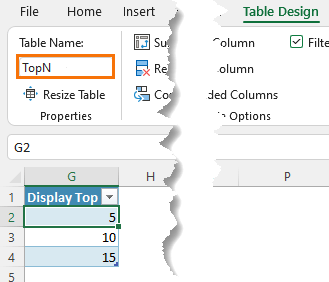
IMPORTANT: These tables are not related in the Power Pivot data model.

Measures to Toggle Top N with Slicers

We need 4 measures:

Measure 1: detects the item selected in the top n slicer:

Selected TopN = MIN('TopN'[Display Top])

We use MIN here to handle the possibility the user selects more than one item in the Slicer. You could equally use MAX if you prefer.

Measure 2: We need to calculate the total amount, which is used in the next measure. It's easy with the SUM function:

Total Amount = SUM(Data[Amount])

Measure 3: Ranks the Sub-categories 1 to n based on the top N selected in the Slicer.

Rank Sub-category = RANKX(ALLSELECTED(Data[Sub-category]), [Total Amount], , 0)

RANKX returns the ranking of all selected sub-categories based on the Total Amount. The last argument, zero, specifies the sort order in descending order.

Measure 4: Filters out the sub-categories we don’t want included using an IF formula:

Include Sub-category = IF([Rank Sub-category] <= [Selected TopN],1,0)

It simply says, if the rank is less than or equal to the selected top n value, then return 1, otherwise return zero.

PivotTable to Toggle Top N with Slicers

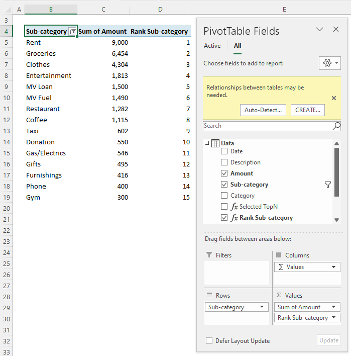
Now we can build the PivotTable to support the Pivot Chart. The PivotTable end result is below (don't worry about the yellow warning in the Field List as this is expected).:

However, to apply the filter we temporarily add the ‘Include Sub-category’ measure to the PivotTable Values area:

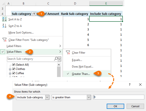
Once the filter is applied, the ‘Include Sub-category’ measure can be removed from the PivotTable.

And sort in ascending order based on the Rank Sub-category field.

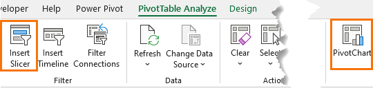
Now you can insert the Slicer and the Pivot Chart:

Pivot Chart Formatting

The Pivot Chart starts off a bit ugly:

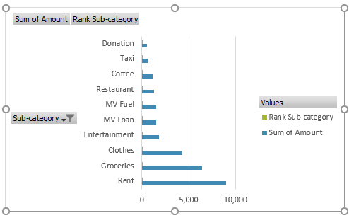
Let’s apply some formatting to pretty it up (see video for further details).

1. CTRL+1 the chart to open the format pane > Format Axis > Axis Options > Categories in reverse order
2. Right-click the field buttons on the chart > Hide all field buttons on chart
3. Select the ‘Rank Sub-category’ series in the chart > set fill colour to No Fill
4. Set the series overlap to 100%
5. Set the gap width to 50%
6. Remove the legend
7. Add custom dynamic chart label referencing another PivotTable that captures the Selected TopN.

Want More

Check out this tutorial that also uses disconnected tables to change the aggregation method using Slicers.

Want to learn more about Power Pivot? Please consider my comprehensive Power Pivot and DAX course.