Slicers enable you to quickly and easily toggle filters on and off. They're best known for working with PivotTables, but Slicers also work with Excel Tables.
I like to use them to save time applying filters I use regularly, but we can also create dynamic reports by leveraging formulas that can recognize when a row is filtered out because of Slicer selections.
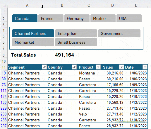
Table of Contents
Watch the Video

Download Workbook
Enter your email address below to download the sample workbook.

Understanding Excel Tables
Excel Tables are not just nice formatting. Tables work as a unit and make updating, using, and analysing data in a spreadsheet easier and faster.
Tables come with default formatting that makes them easy to read:
But they can also have no formatting and blend in with your existing file look and feel:
Why Use Excel Tables
Tables streamline the way you work with your data, making it more efficient to reference, analyse, and maintain with features like:
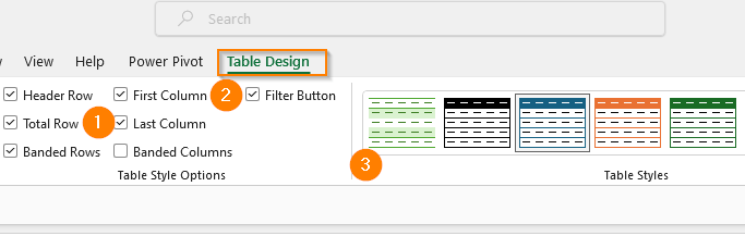
- Easy-Add Totals: The table design menu allows you to add or remove a total row. This row updates automatically as you filter data, without adjusting the formula. Also, you get several formula options for the total, such as sum, average, count, min, max, etc.
- Easy-Add Filter Buttons: By default, all columns in a table get filter buttons that allow you to filter easily. You can disable them from the table design menu.
- Easy-Format Styles: You get several built-in formatting styles to make your data look more attractive. Also, banded rows or columns options alternate fills in rows or columns, so no need to spend hours on formatting!
- Auto-Freezing Column Headers: Tables allow you to scroll down and still see the column headers without needing to freeze the top row. This prevents you from adding data to the wrong columns.
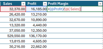
- Auto Named Ranges: Formulas in tables don't reference the cells you add to the formula, they reference the column name, making it much easier to understand what the formula does. For example, if you want to calculate Profit Margin, instead of using cell references, the formula would show Profit/Sales so anyone who checks the formula knows how the value is calculated.
- Auto Formula Copy: On adding a formula to a cell, the formula gets copied down to all the cells in that column without you needing to add it manually for each row.
- Auto Expansion: No more dragging formulas or formatting every time you add new data, tables expand automatically both vertically and horizontally.
- Dynamic Charts: The charts & visuals for your data get updated automatically as soon as you add new data.
If you want to use any of the above options in your table, here is the complete step-by-step tutorial on these features.
Tip: If you haven't already formatted your data in a Table, you can do so by selecting a cell within your data range, and then with the keyboard shortcut CTRL+T or via the Insert tab > Table.
Filtering Data in Tables
Filtering data in Excel tables allows users to quickly locate and analyse specific subsets of data, enhancing the efficiency and accuracy of data analysis by focusing on relevant information and improving the readability of datasets by hiding irrelevant or unwanted rows or columns.
This can be particularly valuable in large datasets where manually sifting through data would be impractical or time-consuming.
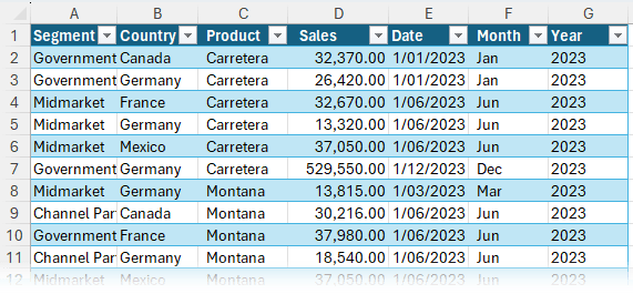
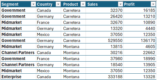
Taking the data below:
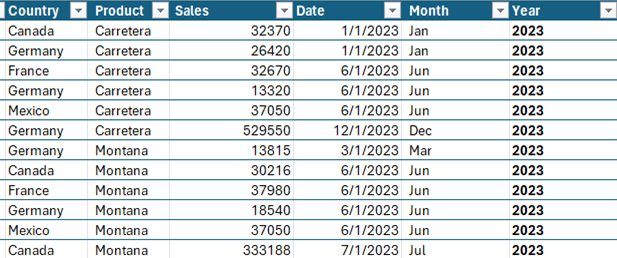
Suppose you have a spreadsheet with the sales data for each month of the year, for 6 products, from 5 countries. But your boss wants you to quickly give them the sales numbers for September, for the product Carretera from France.
Normally, you'd filter the headers of each of these columns, uncheck 'Select All' and then select the desired parameter.
What if there was an easier way to do this? Fortunately, there is, using Slicers.
Explanation of Slicers and their Functionality
A Slicer is a quicker, easier, and more intuitive way to filter data.
In the above example, all you need to do is create Slicers for month, product, and country, and select the relevant values for each of these fields with just 3 clicks. And voila! You have the numbers your boss asked for within seconds!

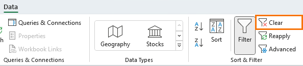
But wait, the magic doesn't just end there, once your boss is done seeing the numbers, you just need to click the clear filters button in the top right of each Slicer to revert your data back to its original state. Or check the clear filters button on the Data tab of the ribbon to remove them all in one go:
Slicers Can Enhance Analysis
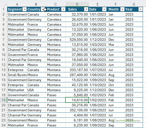
Suppose your data has 2 more columns - Segment and Profit, and you need to figure out which segments are making losses while which are profitable.
You can build PivotTables and charts, or filter the profit column for only negative values, OR use Slicers!
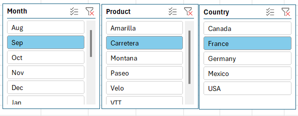
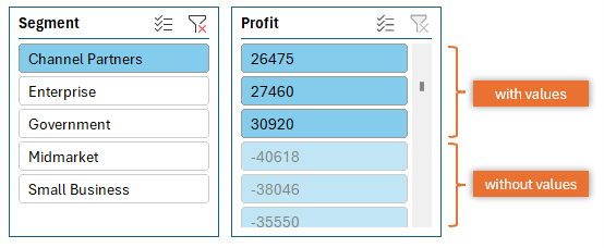
Start by creating 2 Slicers for Segment and Profit.
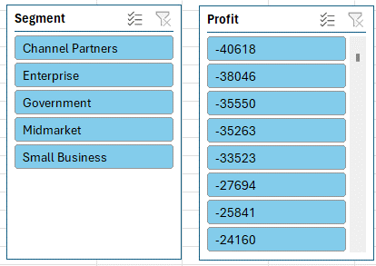
Note: Slicers automatically sort in numerically/alphabetically, which is negative to positive in the case of the Profit Slicer.
Now select any one Segment, such as Channel Partners, and simply look as the first Slicer value in the profit Slicer. Segment Slicer filters your data and all the other Slicers too. Therefore, you will only see those values in your Profit Slicer belonging to the selected Segment.
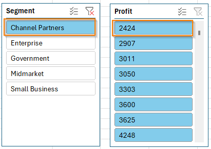
We can see above the first value in the Profit Slicer is positive, the Channel Partner segment is not making any losses.
Click on each Segment one by one to find out which Segment is making losses in just a few clicks.
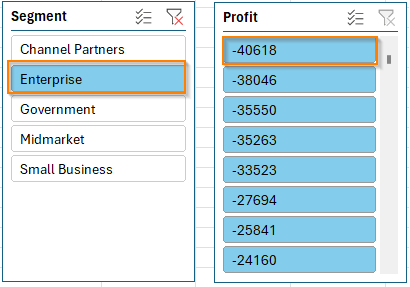
Knowing that the Enterprise segment is the loss-making segment, you can investigate further and take necessary action.
Creating and Customizing Slicers
Before adding a Slicer, make sure your data is in a Table format and preferably without any empty cells in the columns you want Slicers for.
Use any one of the following methods to insert a Slicer.
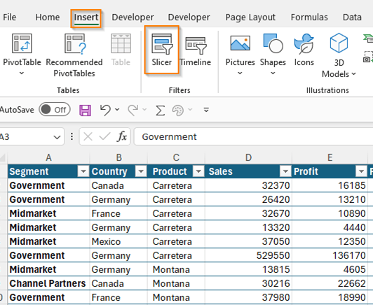
Method 1: Add a Slicer from the Insert Tab
Click on any cell within your Table > Go to Insert Tab > Select Slicer:
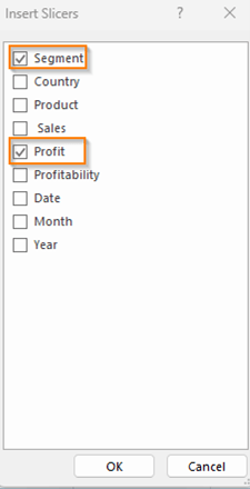
An Insert Slicer window will appear, choose the field (column) you want to filter your data on. You can select multiple fields. Each field will have a Slicer of its own:
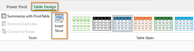
Method 2: Add a Slicer from the Table Design Tab
- Click on any cell within your Table > Go to Table Design Tab > Select Insert Slicer:
The Insert Slicer window will appear, for you to choose a field.
Customization Options for Slicers
Slicers have many formatting options available via the Slicer tab:
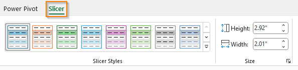
However, they are a bit chunky and take up a lot of space. Unfortunately, many of the most important formatting options are buried. Check out this tutorial on Slicer Formatting for insider secrets on making Slicers really small and more.
How Slicers Interact with Tables
Slicers have several components to help you filter data efficiently:
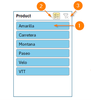
- Selection buttons: Select the desired items by clicking on them. To select multiple items, keep CTRL pressed while selecting them or hold SHIFT to select a range of items.
- Multi-select button: To select multiple items without pressing CTRL, click on the multi-select button on use the shortcut Alt +S. This is handy when working with touch screen devices and can't easy hold CTRL or SHIFT to multi-select.
- Clear filters: Press to undo selection i.e., revert your data to the original state
If you have a lot of items, Slicers will automatically have a scroll bar.
Multiple Slicers Interaction
As hinted in the Segment-Profit example, Slicers filter other Slicers. This property makes filters applied by Slicers additive.
When you select one Segment, the Profit Slicer's scope is automatically reduced. Instead of showing all Profit values, it only shows the Profit values of the selected segment. Data with no values in the current filter state becomes lightly shaded compared to relevant data.
Advanced Techniques
A handy alternative to summarising your data with a PivotTable is to use aggregation functions that ignore filtered rows, like SUBTOTAL and AGGREGATE, to summarise data in response to Slicer selections.
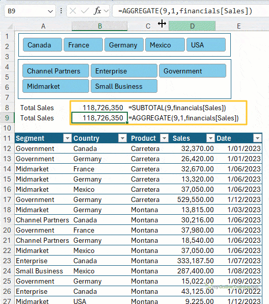
Thanks to Jon von der Heyden for this tip.
Tips and Best Practices
- Consider the order of Slicers on the sheet: Put them in a logical order that leads the user on a journey through the data. e.g. if users are interested in only one region, then put the Region Slicer first.
- Slicer placement: Slicers work independently of the sheet where the Table is stored. Thus, you can simply cut and paste them to a report sheet along with your other visuals.
- Slicers snap to grid: Press Alt while moving multiple Slicers so that they snap to grid while moving them.
- Keep Slicers aligned: Press SHIFT while moving the Slicer vertically or horizontally so that it stays aligned to the starting location on the worksheet.
Limitations of Slicers
- Slicers only connect to one Excel table: You can have multiple Slicers for an Excel table, but you can't use the same Slicer to connect to multiple Excel tables. To use Slicers to filter multiple tables, use multiple Pivot tables instead. Check out this tutorial for more on PivotTables.
- No 'Select All' button: Slicers don't have a 'Select All' button. Although there is a clear filter button that has the same effect. Just note that if you want to remove the Slicer headers to make it look more appealing, you'll have to manually select all values to clear filters.
- Slicers take up quite a lot of space: If left in their default style, Slicers take up a lot of space. Follow the tips in this tutorial on Slicer Formatting mentioned earlier for insider secrets on making Slicers really small and more.
- Multiple Slicers are needed to filter multiple fields: If you have grouped dates in your data in mm-dd-yyyy format, you might need 2 Slicers to filter your data for months and years. To avoid having too many Slicers, create helper columns concatenating 2 or more fields, check out this tutorial on Helper Columns.
Next Steps
Tables can significantly improve efficiency but less than 2% of Excel users know how to use them! Make sure you're getting the most out of Excel with our Excel Tables course.
Or are you ready for PivotTables? PivotTables can seem overwhelming at first, but in our 1.5 hour PivotTable Quick Start course we'll have you up and running and wondering what all the fuss was about as they enable you to rapidly build interactive reports. Spoiler: it's all in getting the data layout right.
Get the insider tips on how to format Slicers in our comprehensive Slicer Formatting tutorial.

If you have hidden the Slicer headers for neatness (always) and have only 1 item selected, then ctrl-clicking that item in the Slicer will clear the filter
Alternatively you can drag-select the full list in the Slicer to quickly clear a multiple filter
Or, when a filtered item is selected in the table, press the context menu button then “E” twice (context menu button = right-click = shift-F10) – works with or without Slicers
Another good tip is context menu button, “E”, “V” to filter a table on the current cell
Thanks for sharing, Jim! I’ve used the others, but not CTRL clicking the button again.
amazing what you find by mistake!
😀
In your article, Slicers for Excel Tables”, Under the section of “Advanced Techniques” you mention the use of SUBTOTAL and AGGREGATE. I like this use of of these formulas to get a total or other statistical measures at the top of the table. Can you do more with formulas like this when using slices to filter an Excel Table. For example, calculating some measure of relatively such as share of all sales or share of sales in a specific country or both?
Hi Bill,
Sure, most functions don’t ignore hidden or filtered rows, so for example, you could calculate percentage of total using SUBTOTAL or AGGREGATE to get the numerator and SUM to get the denominator.
Mynda
Tables and slicers are a great way to produce a dynamic chart, but how do you find out the slicer selection to use it in a dynamic chart title?
Hi Stephen,
If you’re confident that there will only ever be one item selected in the Slicer at a time then you can use this array formula to return the first visible cell in the column of the filtered table:
Remember to enter this with CTRL+SHIFT+ENTER as it’s an array formula.
Mynda
How about using some combination of TEXTJOIN and UNIQUE:
=TEXTJOIN(“, “,TRUE,UNIQUE(B$10:B$2000))
to get over the multiple item issue also perhaps COUNTA for a count of number of items selected in slicer:
=COUNTA(UNIQUE(ExcelTableName[ExcelTableColName]))
Sure, great ideas, Bill. Useful if you have small tables/not many possible items. On larger tables it could return an unwieldy result.
Dear Mynda,
I have an Excel Table and I have a Pivot Table with the Excel Table as data source. Is there any way to use a slicer to control both the Excel and the Pivot table with the same slicer?
Thank you!
Hi Rita,
No, they’re not able to be connected. The PivotTable slicer references data in the Pivot Cache, whereas the Table Slicer references the Table directly, so one Slicer cannot control both….unless you use some custom VBA to mimic the selections from one Slicer to the other.
Mynda
Thank you! It’s a pity but I hope I can find a workaround.
There may be a workaround depending on how you have your data laid out and what you need to see.
I track metrics for one of my manager’s direct reports. I have a table of data that I need to use for charts tracking several employees effectivity rate per month. And to keep it interesting, he wants the chart to show a rolling 13-month time frame.
I have 6 regular tables (one per employee and one for an overall percentage) all lined up side by side. I have a table slicer for the first table. When I select the 13-months I want to track, all 6 of my tables are filtered – because they are side my side. I added a pivot table (using months as the row label) in beside the tables and when I filtered my tables, it too was filtered.
I tried inserting a pivot chart thinking that would also change but it doesn’t. Apparently pivot charts are smart enough to know the difference between not being able to be seen and filtered. Darn it.
Clever twist, JoAnn 🙂
There is a little bit of confusion in this post. Slicers became available for pivot tables in Excel 2010, however, they can only be used in tables with Excel 2013. Much to my disappointment. I love slicers.
🙁 sorry about that JoAnn. I’ve updated the ‘note’ to include this. Pray for Excel 2013…or wait for Excel 2016 which will be out this year!