Relative Named Ranges

Excel Named Ranges is a vast topic that includes some simple techniques that we all can and should use to make our spreadsheets easier to build and maintain. Plus, some more advanced techniques like relative named ranges, which are good to know. Especially for that occasion when you inherit a workbook from an Excel Superuser who thinks you’ll have no hope deciphering their file.

Note: If you’re not familiar with Named Ranges you can read up on them here first.

Download the Workbook

Watch the Video

Relative Named Ranges

A Relative Named Range returns a result that is relative to the cell in which you use it. As opposed to regular named ranges which are typically absolute, in that it doesn't matter where you reference the named range from, it will always return the same result.

To understand this let’s take a moment to revisit a concept that every Excel user should know very well, and that is the way a relative cell reference automatically updates as it’s copied from one cell to the next.

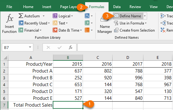
For example, cell B7 in the image below contains a SUM formula that uses relative cell references B2:B6:

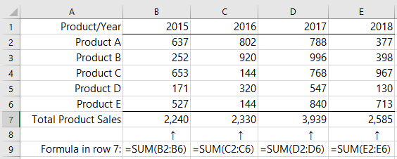
When we copy the formula in cell B7 across to cells C7, D7 and E7 it automatically adjusts the column reference relative to its new location. i.e. copying the formula in B7 across one column to cell C7 will result in =SUM(C2:C6), and so on.

Note: If I were to copy the formula down a row the row references would also adjust as they are also relative. More on relative and absolute references here.

Relative Named Ranges work in the same way, and we can use them to replace the individual SUM formulas in row 7 of the example above.

For example, in the image below, row 7 contains the formula =Total_Sales. The Edit Name dialog box shows that the name Total_Sales, which is displayed for the active cell, B7, is referring to the formula:

=SUM(Sheet2!B2:B6)

Total_Sales is in essence a named formula, and I’ll refer to it as such going forward.

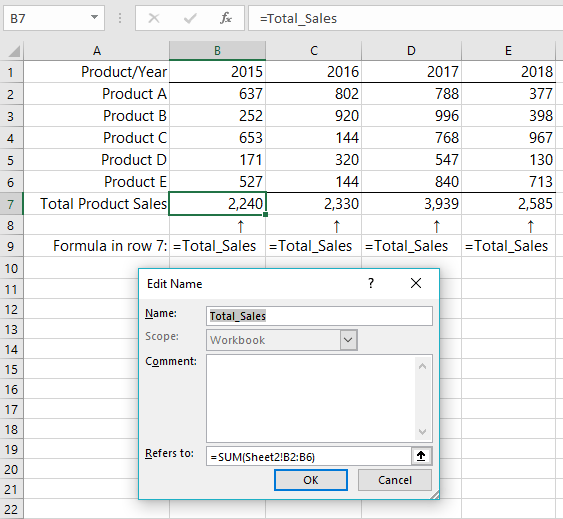
Notice that the named formulas in cells B7, C7, D7 and E7 are all the same; =Total_Sales

However, if I edit the name while the cursor is set in cell C7 you can see in the image below that the named formula, Total_Sales is now referring to cells C2:C6:

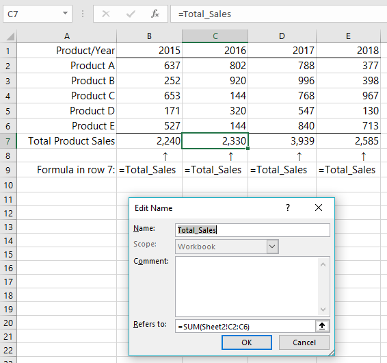
Likewise, if you edit the names while cells D or E are selected. In other words, the named formula Total_Sales will always sum the 5 cells immediately above the cell in which you place it. It does this because the cell references in the Refers to field are relative.

Scope of Relative Named Ranges

The named formula, Total_Sales, has the scope of the workbook, meaning I can use it on any sheet, however the formula in the Refers to field (see image below) specifies that it will always sum cells on Sheet2:

For example, if I enter =Total_Sales in cell B7 on sheet 1 it will sum cells B2:B6 on sheet 2.

If I want to use this named formula relative to any sheet, I can change it to:

=SUM(!C2:C6)

Omitting the sheet name and leaving the exclamation mark in front of the cell references results in a dynamic sheet reference. So, while the named formula will have the scope of the workbook, it will refer to the active sheet.

For example, now if I enter =Total_Sales in cell B7 on sheet 1 it will sum cells B2:B6 on sheet 1.

In other words, I have a truly relative named formula, i.e. relative to both the cells and the sheet.

Warning: This use of an exclamation mark in named ranges has been known to cause Excel to crash and can create problems when used with VBA (e.g. creating an action like Application.CalculateFull), so use it with caution. That said, I’ve never experienced any problems, so it may be resolved in more recent versions of Excel.

Relative named ranges and formulas should be used with care, because if you use them in the wrong location they can still return results, but they may be invalid simply because of the cell you use them in.

Creating Relative Named Ranges

Location, location, location. It’s the cliché that should be front of mind when creating relative named ranges.

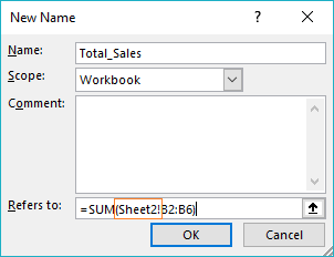
When you create a relative named range, you should first select the cell that you want the range relative to. For example, to create the Total_Sales named formula I first selected cell B7. Then Formulas tab > Define Name:

This will open the New Name dialog box where you can give your named range or formula a name (no spaces allowed), select the scope and enter the cell reference or formula in the Refers to field:

Other Uses for Relative Named Ranges

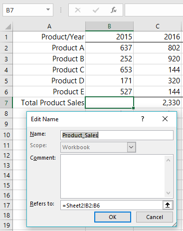
So far, the example we’ve looked at is a relative named formula, but you can also create a relative named range. For example, with cell B7 selected we can name the cells B2:B6; Product_Sales:

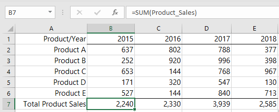
And then use the relative named range in a SUM formula (or any other formula):

Relative Dynamic Named Ranges

Dynamic named ranges are a staple for the intermediate/advanced Excel user. They allow us to return a range that adapts to ever changing data. For example, we might use a dynamic named range as the source for a PivotTable.

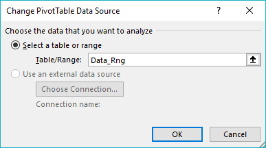
As new rows are added to our source Data_Rng, the dynamic named range also increases to include the new data, thus eliminating the need for us to update the PivotTable data source cell references.

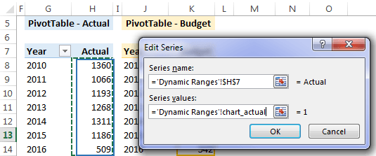
Or maybe you’re using a PivotTable as the source data for a regular chart. You can use a dynamic named range for the chart source allowing it to automatically pick up changes to the PivotTable size.

However, typically these dynamic named ranges aren’t relative.

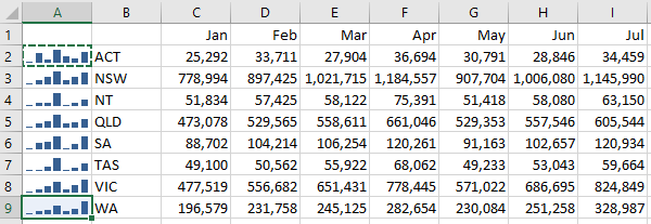
An area where relative dynamic named ranges will come in handy though, is for Sparklines. In the image below, I’ve inserted a group of Sparklines in column A and you can see the Data Range is hard coded C2:I9:

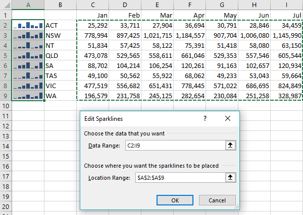
This means that when new data is added for future months in column J onward, we’ll have to edit the Sparkline Data range and update it… MANUALLY! That ‘M’ word is enough to make an advanced Excel user queasy.

Now ideally, we’d use a dynamic named range for the Sparkline Data Range, but you can’t enter a dynamic named range for a Group of Sparklines, only for individual Sparklines. And I don’t fancy creating 8 separate dynamic named ranges. That’s way too much work.

Luckily, we can create one dynamic named range that is relative to the cell it’s in and use that for each individual Sparkline (it’s a lot quicker to copy and paste 8 Sparklines).

With the Sparklines removed, I’ll start with cell A2 selected > Formulas tab > Define Name.

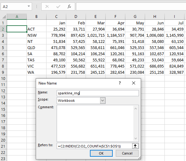
I’ll call my relative dynamic named range ‘sparkline_rng’, and use an INDEX formula like so:

=C2:INDEX(C2:O2,,COUNTA($C$1:$O$1))

In English it reads;

Start the range in cell C2 and find the last cell in the range C2:O2 using INDEX, skip the row argument for INDEX because there's only one row being INDEXed, then COUNTA returns the column number argument by counting the columns that contain text in the range C1:O1 to find the last column containing a month name.

Create a named range for the Sparklines; I called mine sparkline_rng as you can see below:

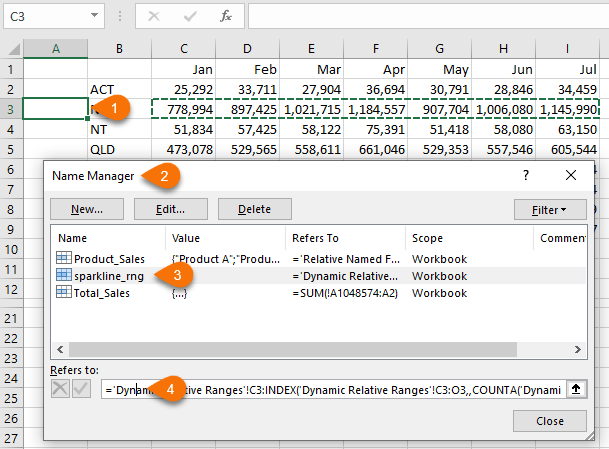
I can check the formula is evaluating correctly by inspecting it in the Name Manager (CTRL+F3).

For example, in the image below, you can see I’ve selected cell A3 (1) and in the Name Manager (2) I’ve selected the sparkline_rng in the list of names (3). To see the marching ants around the cells returned by the formula, I simply click anywhere in the ‘Refers to’ box (4):

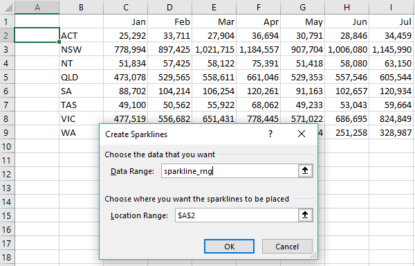
Now that I know my named range is working correctly I can insert the Sparklines. Just enter the first one and in the Create Sparklines dialog box enter the relative dynamic named range in the Data Range field:

Then copy and paste the Sparklines one at a time, so they remain ungrouped:

A big thanks to Christopher Mangels for the Sparkline example.

Limitations

Relative named ranges cannot be used in hyperlinks because cell A1 is always the hyperlink anchor for a defined named:

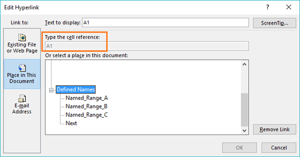
Using absolute named ranges with Hyperlinks isn’t an issue, but for relative named ranges it essentially renders them absolute, or always relative to A1 when used with hyperlinks.  If someone knows how to circumvent this, please let me know as it has been driving me crazy!

Name Range Manager

If you are in need of a utility to manage defined names in your Excel models, this one is a must-have.

• List all names in your active workbook.
• Filter them using 13 filters, e.g. "With external references", "With errors", Hidden, Visible.
• Show just names that contain a substring.
• Show just names unused in worksheet cells.
• Edit them in a simple dialog or make a list, edit the list and update all names in one go.
• Delete, hide, unhide selected names with a single mouse click.