In this post I’m going to show you how to use Power Query’s Unpivot tool to fix 3 common data layout problems:
- The Straightforward Unpivot
- Unpivot Multi-column Data Types
- Unpivot Nested Column Headers (the worst offender):
- And to flip things around, literally, we’ll use the Pivot tool to fix Repeating Rows, which is commonly referred to as Stacked Data.
While all those examples are amazing, the icing on the top is that the query retains a link to the original data (blue tables), so should any of it change, you can simply refresh the query and the green tables get updated too.
Watch the Video

Download the Workbook
Enter your email address below to download the sample workbook containing step by step written instructions:
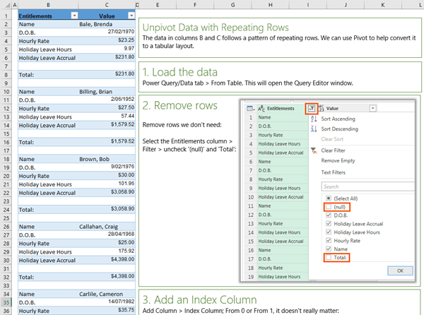
Figure above - Excel workbook with step by step instructions
Power Query Unpivot Scenarios - Written Instructions:
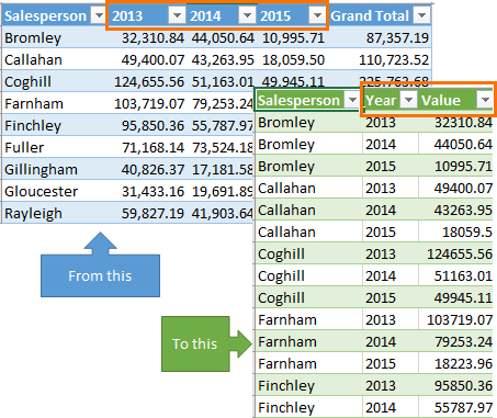
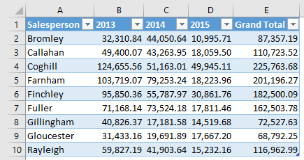
Straightforward Unpivot
In this example we want to unpivot columns B:D and remove the Grand Total, in column E.
Tip: Format the data in an Excel Table first and give it a useful name.
- Load the data into Power Query: Excel 2010 & 2013 Power Query tab/Excel 2016 - Data tab > From Table. This will open the Query Editor window.
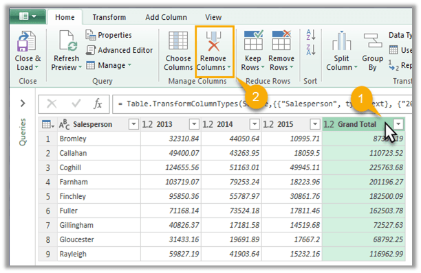
- Remove the Grand Total column: Left click to select it and press the Delete key, or go to the Home tab > Remove Columns, as shown below:
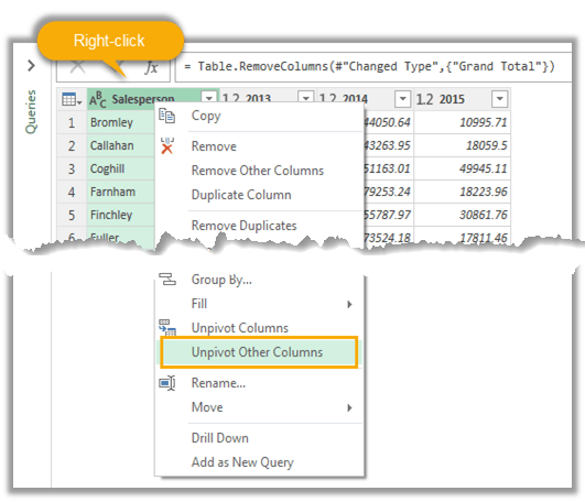
- Unpivot the year columns: select the Salesperson column > right-click > Unpivot Other Columns:
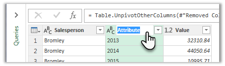
- Rename Columns: double click the Attribute column header and enter a new name; Year:
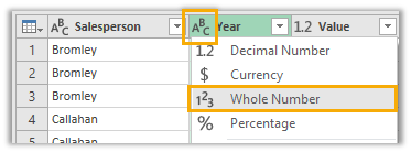
- Change Type for Year column: Click the ABC icon in the Year column header > select 'Whole Number':
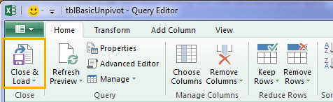
- Close & Load: now you're ready to load the data back into the Excel worksheet. Click the 'Close & Load' button on the Home tab:
Tip: Click the drop down arrow on the Close & Load button and choose ‘Close & Load To’ for more options on where to load the data.
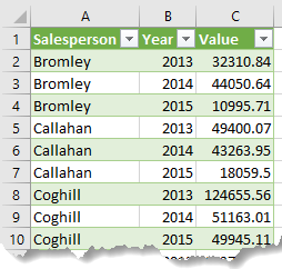
Voila! Now you can create your PivotTable reports using data correctly formatted in a Tabular layout:
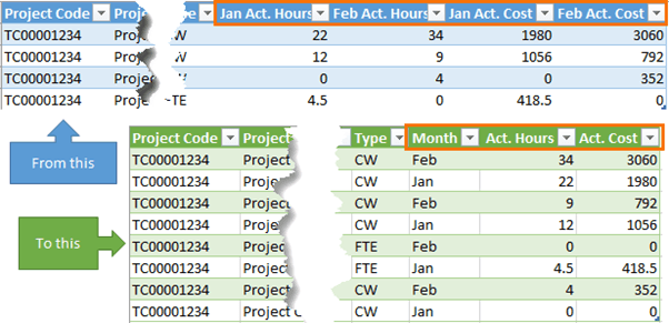
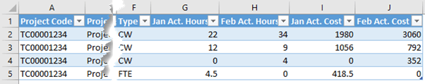
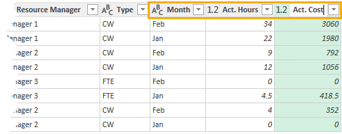
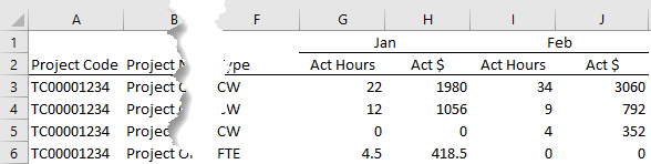
Multi-column Data Types
In this example we want to unpivot columns G &H (hours) and I & J (cost) separately.
- Load the data: Excel 2010 & 2013 Power Query tab/Excel 2016 - Data tab > From Table. This will open the Query Editor window.
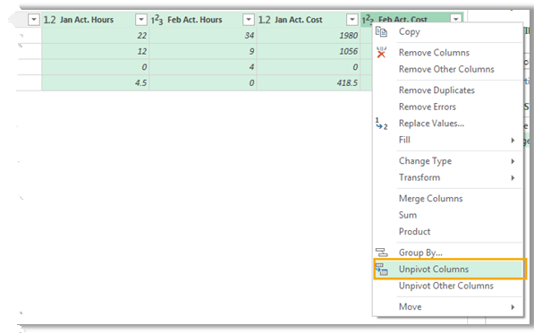
- Unpivot the Values Columns: select the 4 columns containing values > right-click the column header > Unpivot Columns:
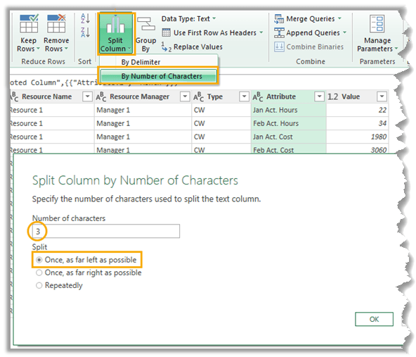
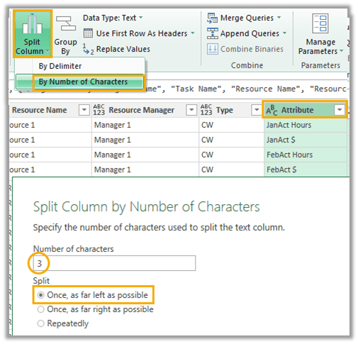
- Split Attribute Column by Number of Characters: Select the Attribute column > Home tab > Split Column > by Number of Characters.
In the dialog box enter 3 (this will split after the month name) > Split; Once, as far left as possible:
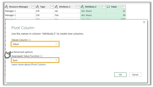
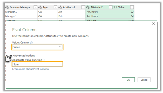
- Pivot the Attribute.2 and Value Columns: This will put the Hours and Costs values into separate columns.
Tip: Select the Attribute.2 column first, then select the Value column > Transform tab > Pivot:
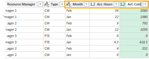
- Rename Columns: double click the column headers and rename as required:
- Close & Load: now you're ready to load the data back into the Excel worksheet or data model etc.
Nested Column Headers
In this example we want to unpivot columns G to J, but the headers are split over rows 1 and 2.
- Format in Excel Table: select the data including the headers > CTRL+T to format as an Excel Table. Uncheck 'My Table has headers'.
- Load the data: Excel 2010 & 2013 Power Query tab/Excel 2016 - Data tab > From Table. This will open the Query Editor window.
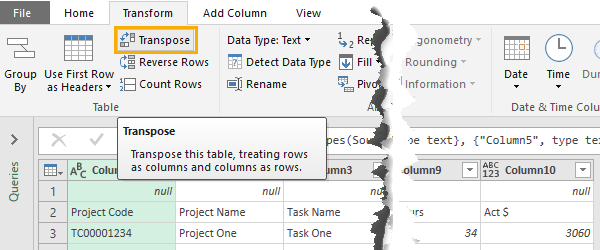
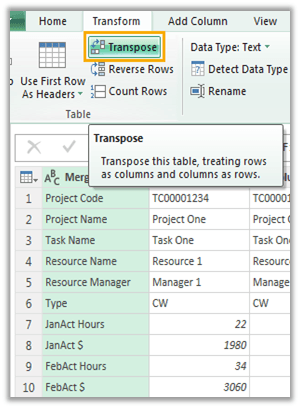
- Transpose Table: Transform tab > Transpose:
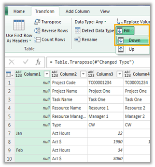
- Fill Down Month Labels: select Column1 > Transform tab > Fill Down. This will repeat the month names on each row where relevant:
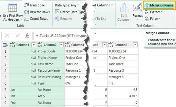
- Merge Columns: merge columns 1 and 2. I won't use a delimiter because the month values in Column1 are all 3 characters long, so I can easily split the column by length later.
- Transpose: transpose the table back to its original layout:
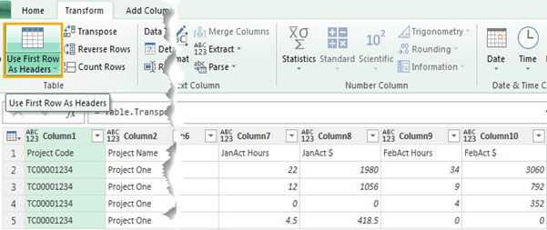
- Promote First Row to Headers: now that the column labels are in one row we can promote them to the header. Transform tab > Use First Row as Headers:
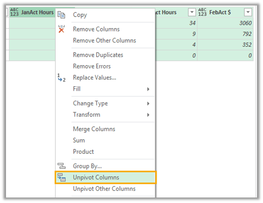
- Unpivot the Values Columns: select the 4 columns containing values > right-click the column header > Unpivot:
- Split Attribute Column by Number of Characters: select the Attribute > Home tab > Split Column > by Number of Characters.
- Pivot the Attribute.2 and Value Columns: This will put the Hours and Costs values into separate columns.
- Rename Columns: Double click the column headers and rename as required:
- Close & Load: now you're ready to load the data back into the Excel worksheet or data model etc.
This enables us to join the two header rows together because transposing them will put them into columns, which can be joined, but first…
In the dialog box enter 3 (this will split after the month name) > Split; Once, as far left as possible:
Tip: Select the Attribute.2 column first, then select the Value column > Transform tab > Pivot:
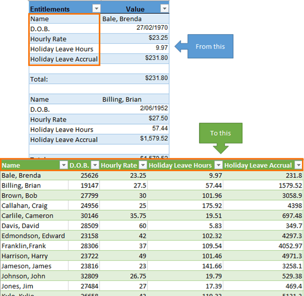
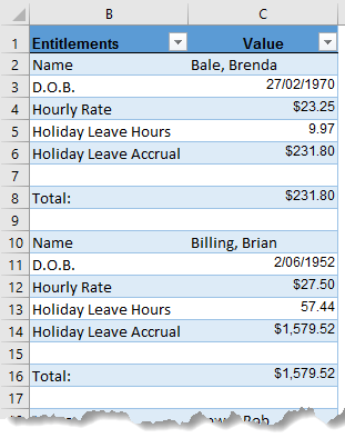
Repeating Rows
The data in columns B and C follows a pattern of repeating rows. We can use the Pivot tool to help convert it to a tabular layout.
- Load the data: Excel 2010 & 2013 Power Query tab/Excel 2016 - Data tab > From Table. This will open the Query Editor window.
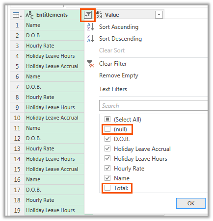
- Remove rows we don't need: Select the Entitlements column > Filter > uncheck ‘(null)' and 'Total':
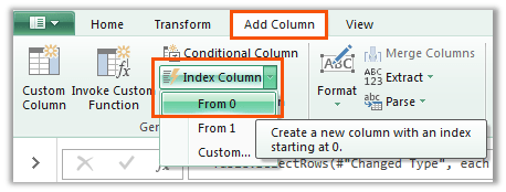
- Add an Index Column: Add Column > Index Column; From 0 or From 1, it doesn't really matter:
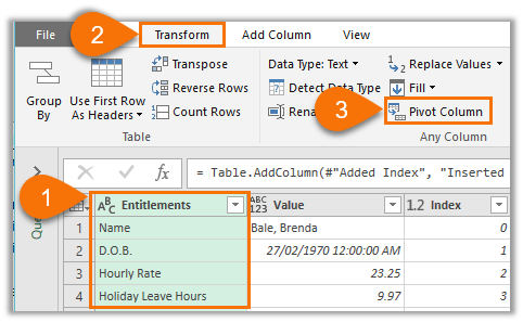
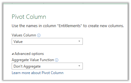
- Pivot the Value column: select the Entitlements column > Transform tab > Pivot Column:
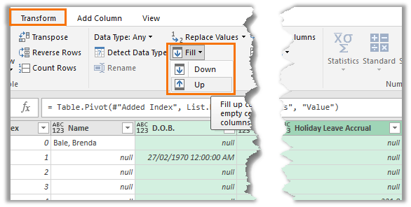
- Fill Up: select the D.O.B. through to Holiday Leave Accrual columns > Transform tab > Fill Up:
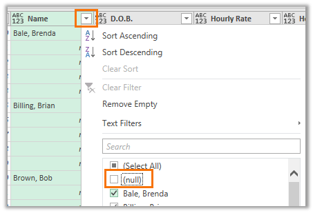
- Filter Name Column: remove the null rows. This will remove all the rows that we don't need, leaving us with just one row per person.
- Delete Index Column: we don't need the Index column anymore. Select the headers and press the Delete key.
- Close & Load: now you're ready to load the data back into the Excel worksheet or data model etc.
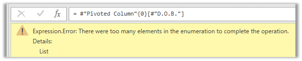
Tip: The reason we add an index column is so that when we Pivot the data in the next step, we don't get the very unhelpful “Expression Error: There were too many elements in the enumeration to complete the operation”. This error can be triggered by duplicate values in the column being pivoted.
In the Pivot Column dialog box under 'Advanced Options' select 'Don't Aggregate':
More Power Query
I bet you can’t wait to use Power Query!
Firstly, you may need to install the Power Query add-in. Click here to see which versions of Excel support Power Query and where to download and install it.
Then read more Power Query tutorials.
And if you want to get up to speed quickly, please check out my Power Query course.
Thank you for this unpivot discussion! I’m working with a table that have a series of columns titled with Category*Year as the title with a value in the cell and wondered if you might point me in the right direction. I am trying to get this info into tabular form. Ideally, I could convert this into Date, Category and Value columns. There are four different Category Names along with up to 9 years with each category. I was trialing unpivoting each of the 4 categories of columns but found that the number of rows is expanding quickly with each successive unpivot. There are hundreds of rows in my table to begin with. Do you have any recommendations? Do I need to add an index row/column so that different dates and categories can be grouped into their respective columns (as opposed to a unique column for each which is what occurs when unpivot is done serially)? Alternatively, I was reading about List.zip and wondered if that might be applicable here?
Hi Steve,
It’s difficult to picture your data. Please post your question on our Excel forum where you can also upload a sample file and we can help you further.
Mynda
Please disregard this question. I realized that I was over complicating the solution. Since there is only one value in each cell, I realized that one can unpivot any number of columns and and then parse the categoryxyear into separate columns after the data is unpivoted (as opposed to reversing these two steps). Your material is very helpful in any case! Best Regards
you are the most flipping amazing content creator, probably one of the best I’ve seen on youtube. And god damn it if it’s a compliment. Thank you for your help!
Wow, that’s incredibly kind of you! Thanks for taking the time to leave your comments. I’m so pleased you found my videos helpful.
How could I do a sunburst table with excel?
Thanks
Please see this tutorial for Sunburst charts.
Hi –
The file download for the Power Query Unpivot Scenarios does not work. When I click on the link to nothing happens; it does download.
Best Regards,
Janet
Hi Janet,
the download link works fine for me. Perhaps your browser or anti-malware is blocking the link. Are you getting any notifications in your browser? Try a different browser.
Regards
Phil
Power Query Unpivot Scenarios – Written Instructions:
I do not find the link for the excel file
The link is under the video. See heading ‘Download the Workbook’ and follow the instructions. Let me know if you’re still stuck.
The download doesn’t work despite trying several times.
Hi OZ,
How exactly does it ‘not work’? It works fine for me. If you enter your email address and click the Get Workbook button, I can download an Excel spreadsheet from the link that is revealed.
This does require JavaScript to be enabled in your browser. Perhaps you have it disabled?
Regards
Phil
Mynda: Absolutely stunning. This was the last of your free offerings I wanted to complete as I start your first two formal courses – boy am I looking forward to those.
Steve
So pleased it will be helpful to you, Steve!
https://drive.google.com/file/d/1Snx_MqEOlRIkj1Yqjw1QsMk6bYP4xcow/view?usp=sharing
I uploaded a .PDF file in the above link. I would like some help to transform (UNPIVOT) the table on the uploaded file in a database, with the fields:
YEAR MONTH VALUE
I read the help in (https://www.myonlinetraininghub.com/power-query-unpivot-scenarios) but I didn’t find out a similar model.
If someone could give a hand I would be very grateful (from Brazil).
Hi Jose,
Please post your question and sample Excel file on our forum where we can help you further: https://www.myonlinetraininghub.com/excel-forum and also share a file with our solution.
Thanks,
Mynda
Thank you so much.
Our pleasure, Adeo!
Hi,
Loved your tutorial.
Is there any way to retain the original table, so that the visualizations crated from my original table remain intact? And table created after using “unpivot selected columns” is created as a separate table?
The original table isn’t altered. Power Query loads the data into a new table.
That is amazing!
I was familiar with the straightforward unpivot but when I had two different attributes (Value and Profit), I thought there was no easy way to proceed – and so did the web, with only the straightforward option appearing in my searches…
…until I came here – and I couldn’t believe how easy it was (though I suspect some form of sorcery is involved)
thanks Mynda for demonstrating so clearly
jim (now happily moved to a company with 365)
Glad I could help, Jim 🙂
I imagine you’re very pleased to now have Office 365.
Hi, really nice post.
I am having a problem to pivot the columns. I am having this error:
DataFormat.Error: Valor de célula inválido ‘#N/A’.
Any ideia what can be ?
Hi Arthur,
One of your cells from the source data has a formula that returns an error. Clear that error in the source.
Thank you for the tutorial!
So I have several columns of revenue by month and several columns of unit sales by month. I’m not understanding how to unpivot both the revenue and the unit sales without them both ending up in the same column, rather than having a revenue column and a units column when I’m done.
Thanks!
Hi Cheri,
Please post your question and sample Excel file in our Power Query forum where we can help you with a detailed response.
Thanks,
Mynda
Thank you for the tutorial! Is there any way that I can apply this query to other sheets in the work book that are all formatted exactly the same?
Thanks!
Hi Matt,
Yes, you can copy the query and then edit it via the Advanced Editor to point at the different sheets.
Mynda
Thanks for this. Assuming I have unpivoted my data and am using the table now. If I add in some columns to the source data table, how do i include these in the unpivoted data table now? I cant figure out to do this using the edit.
Thanks!
Hi Stephen,
If you selected the columns you wanted to keep and then ‘unpivoted other columns’, you could simply refresh your query and it will pick up the new data.
Mynda
Thank you! You have no idea how much you saved me 😀
🙂 you’re welcome, Clara. Glad Power Query was a big help.
Hi, I would like to know more about pivot and unpivot columns and how does it work the INDEX when we got several columns.
greetings!
Hi Carlos,
The reason we add an index column is so that when we Pivot the data, we don’t get the “Expression Error: There were too many elements in the enumeration to complete the operation”. This error can be triggered by duplicate values in the column being pivoted.
Mynda
Your article came to me as a coincident. I saw a tutorial on the same subject on power query but very confusing as there is no example on how to apply it, wow, it was very painful as I have developed interest in that subject.
So when suddenly I saw your article complete with the hows, I have nothing but to thank you very much from the bottom of my heart.
Big Thanks again
Hi Uche,
Glad you found this post answered your question. Have fun with Power Query, it’s an amazing tool.
Mynda
Tahnk you Mynda for sharing, and as always, it is a real pleasure to follow your tutorials
Thanks, Mehdi. Glad you enjoyed it 🙂
I don’t have enough words to say how interesting and original is this tutorial, wow, I am so impressed with all that can be achieved with the adequate knowledge, excellent work Mynda!! I feel so identified with the figure 2 “original data” because that’s the way we usually organize time series of data in my office. I am sure this tutorial will create a revolution between my coworkers, I will forward it to my colleagues right now. As you said, I can’t wait to install Power Query, it’s a well hidden diamond!!
You were truly the Angel for that man, he will never forget your help and you gained a loyal friend forever! 🙂 You made his day! It was a pleasure to read this tutorial, your comments were very funny. I smiled a lot while reading it :):)
Thank you, Juan! I’m so pleased you found the unpivot tutorial helpful and enjoyed my story (shared in my Newsletter) 🙂
Thank you for this very informative tutorial.
Thanks, Joan! Enjoy Power Query Unpivot 🙂
Fantastically helpful as ever. I used to think pivot tables were the business until I came across unpivoting!
However, my personal disaster area is unpivoting other people’s multi-column tables where the people have put all the different months or locations on different worksheets. Is there a snappy way to do unpivot those? (preferably with Excel 2010)
Great to hear you’re enjoying Power Query. Of course it can consolidate data spread over multiple sheets and workbooks. There is an example here: Combine Excel worksheets using Power Query
Hope that helps.
Mynda