With the cost-of-living crisis affecting everyone, it's essential to get control of your finances.
Having a personal budget can be your most valuable tool, but creating a budget spreadsheet from scratch can be intimidating, time-consuming, and, for some, a downright chore.
In this post I'll step you through creating a personal budget in Excel, that's not only fun to make, but the results will ensure you stay on track and help you achieve your savings goals.
Don't have time to create a file yourself? Download this template from the link below and watch the video to ensure you understand how to customise it for your own needs.
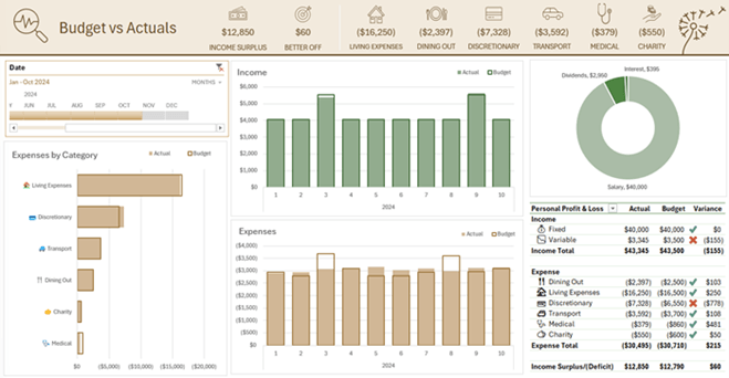
Table of Contents
- Step by step video
- Download Personal Budget Template
- Creating a Personal Budget Template
- Step 1: Identify the types of income and expenses you have
- Step 2: Define a Named Range for the Subcategories
- Step 3: Prepare your budget
- Step 4: Track your actual income and expenses
- Step 5: Prepare Data
- Step 6: Create the Data table
- Step 7: Clean and Transform the Data
- Step 8: Analyse & Visualise the Data
- Automate Gathering Transactions
Watch the Step by Step Video

Download Personal Budget Template
Enter your email address below to download the template.

Creating a Personal Budget Template
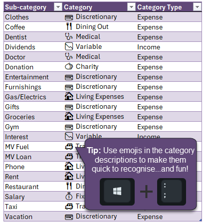
Step 1: Identify the types of income and expenses you have
- List them in column labelled sub-category.
- Then add a column to organise the sub-categories into larger Category groups. This will help you analyse your spending.
- Lastly, add a column to tag the categories as Expense or Income.
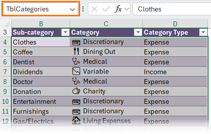
- Format the data in an Excel Table (CTRL+T) so it's easy for Excel to reference and any sub-categories you add are automatically available elsewhere in your template.
- Rename this table: TblCategories:
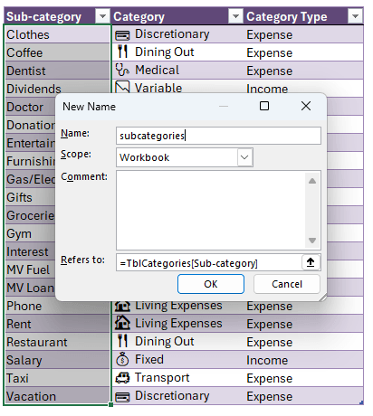
Step 2: Define a Named Range for the Subcategories
Select the Sub-category cells in the table > Formulas tab > Define Name. I've named mine 'subcategories' and you can see it refers to the table's 'Sub-category' column:
Note: in earlier versions of Excel you cannot use the table's structured references in the 'Refers to' field. Instead see this post on Excel Tables as a Source for Data Validation Lists for a solution.
Step 3: Prepare your budget
On a new sheet create a table that estimates values for each income and expense subcategory by month:
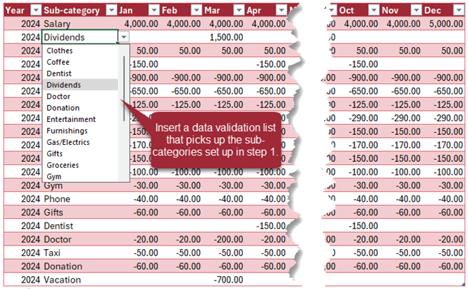
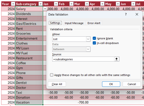
To insert a data validation list, select the cells in the sub-category column of your budget table > Data tab > Data Validation. In the dialog box select 'List' from the 'Allow' drop down menu and in the 'Source' field insert the name of your sub-category list you defined in step 2:
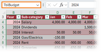
Rename this table, TblBudget:
Tip: Tables are a great way to improve productivity because they make it quick and easy for Excel to reference your data in formulas and PivotTables. When new data is added to a table it's automatically included in anything referencing it, you don't have to edit any references to them. There are a load more useful features available with Tables. Get up to speed with my Excel Tables course.
Step 4: Track your actual income and expenses
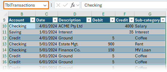
Copy and paste the transactions from your bank statement into a new table. Add the Account and sub-category for each line. Again, use a data validation list for the sub-category field to ensure you have a consistent list of sub-categories.
Remember a Debit is money you spend. i.e. the bank debits your account. A Credit is money you receive e.g. the bank credits your account when you receive your salary.
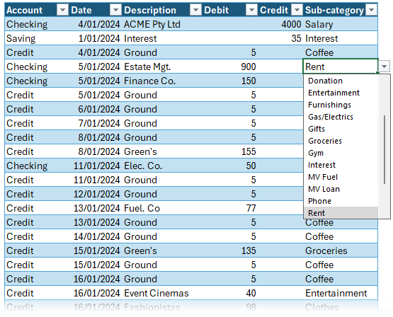
Rename this table, TblTransactions:
Note: if you don't intend to build this budget file for yourself, you can skip this next section and jump to Step 10.
Step 5: Prepare Data
This will enable you to perform calculations on the data without needing formulas that have the potential to break. It sounds scarier than it is, but trust me, this is easy and will make your report bullet proof.
The last thing you want is a formula error telling you that you have more money than you do!
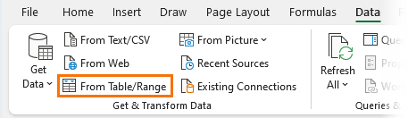
Select the first table, then on the Data tab of the ribbon > From Table/Range:
Then from the Power Query editor window Home tab > Close & Load to… > Only Create Connection:
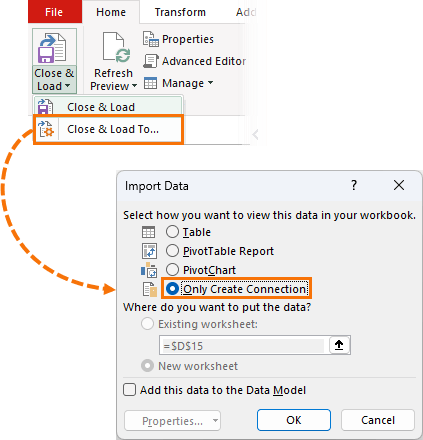
Repeat for the Budget and Transactions Table.
Step 6: Create the Data table
In this step we'll merge the actual and budget amounts into one table and add columns for the Category and Category types to facilitate the reports that will give you insights to your spending.
Note: For detailed step-by-step instructions, see the video above.
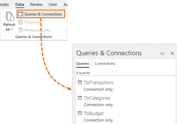
Open the Budget query created in the previous step. Go to the Data tab > Queries & Connections. This opens a task pane on the right. You should have 3 queries listed, one for each of your tables:
Step 7: Clean and Transform the Data
Step 7.1: Starting with the Transactions query, we need to perform the following steps:
- Replace the 'null' values in the Debit & Credit columns with 0
- Add a column to merge the debits and credits into one column and convert the debit amounts to negative values.
- Remove the Debit & Credit columns, as these are no longer required.
We could have done this with formulas, but like I said, formulas are easily broken.
Step 7.2: Next, go to the Budget query and perform the following steps:
- Unpivot the month columns
- Merge the Month name and Year columns and name the new column, Date
- Convert the Date column to a 'date' data type
- Rename the 'Value' column to 'Budget'
This converts the Budget table into the correct tabular layout required to quickly and easily analyse data in Excel.
Step 7.3: Lastly, append the transactions and budget queries together into a new table (Append > as new).
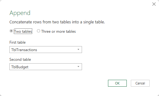
This new query table will be called 'Data'.
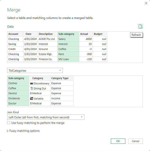
Then merge the Data table with the Categories table to bring in the Category and Category Type fields:
Expand the TblCategories column to bring in the Category and Category Type fields:
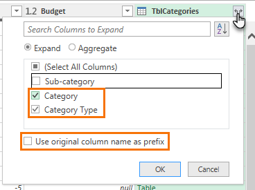
Tip: this is the equivalent of a VLOOKUP or XLOOKUP!
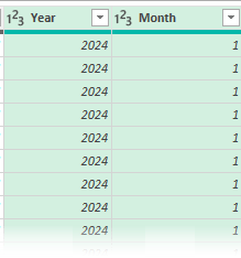
To support the reports, I'll add columns for the year and month numbers. Note: this is because I can't group the dates in the PivotTable
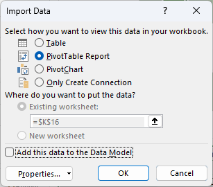
This time I'll Close & Load to… > a PivotTable report.
Tip: 10x productivity and automate more of your boring data gathering and cleaning tasks with Power Query. Get up to speed with my Power Query course.
Step 8: Analyse & Visualise the Data
Now that you've done the hard work of preparing a budget and entering your actual income and expenses, it's time to track how you're doing.
It's super rewarding to see your spending come under control and your savings grow right before your eyes.
You can use PivotTables to summarise your data and compare your actual results to your budget. See the video above for step-by-step instructions.
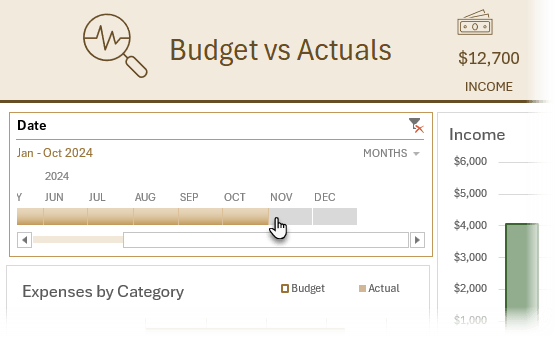
Headline figures give you an up to date view of your position by category and whether you're over or under budget overall:

Use Icons to visually represent the different key figures making them quick to identify and interesting to look at.
Expenses by Category using a bar chart enables you to see which categories are over or under budget and the size of spend in relation to other categories:
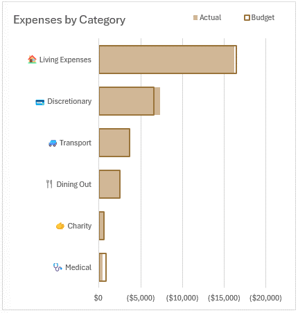
Notice the emojis feed through to the chart axis labels? see, I told you it would be fun!
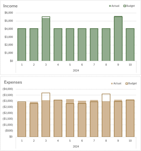
Income and expenses by month allow you to see which months are over or under budget and any trends in your spending which will help you budget in future years:
Income by category allows you to see what proportion each income stream is of your total income. The more you can diversify your income, the less risk you have if any one income stream reduces:
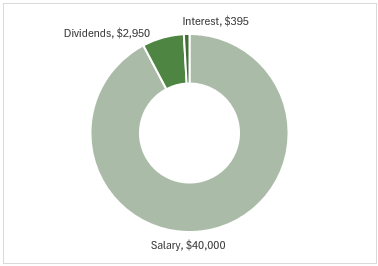
Diversification tip: get a side hustle!
Your Personal Profit and Loss statement allows you to see how each category is performing and your overall position:
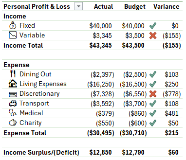
Conditional formatting gives you visual indicators for each category.
Tip: double click on any of the values in the Profit and Loss statement to see the underlying transactions.
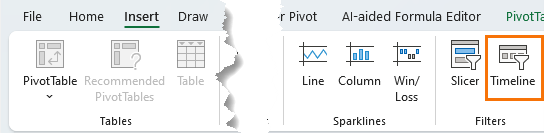
Lastly, insert a Timeline Slicer to filter the charts and visuals for the periods you want to focus on:
Tip: you can use these skills to wow your colleagues at work with interactive reports. Get your skills up to speed quickly with my Excel dashboard course.
Automate Gathering Transactions
To further automate maintaining your budget report, you can use Power Query to gather your bank transactions.
A lot of banks will export transactions to CSV or Excel files and we can use Power Query to automatically get those files from a folder and merge then into a table.
So, check out this Combine Files From a Folder tutorial next.


Hello. just want to ask how can I change the $ in the cells into Peso Symbol? Thank you.
On the Home tab of the ribbon, click on the currency sign drop down and choose > More accounting formats. You’ll find it in there.
Hi Mynda,
You may have already answered this but I am getting an “inconsistent Formula” error when I overwrite the budget numbers in your sample; or I add new lines to the budget sheet – the month columns show a “=REF!” error. (formula is =#REF!/12)
Can you please help?
Hi Mike,
You can ignore the inconsistent formula errors. It’s just Excel expecting you to use the same formula in a whole column, but we are using the table in a horizontal layout where our formulas go across the rows.
The #REF! errors are caused when you delete a cell the formula was relying on. If you’re still stuck, please post your question on our Excel forum where you can also upload an Excel file and we can help you further.
Mynda
Thank you for this tutorial! This was extremely helpful. Quick question – when starting the new year, how to do you change the Report tab to only focus on the new year vs both 2024 and 2025?
Great to hear, Maggie. You can add a Slicer for the Year field and filter your report to only show data for 2025.
When I add the new year budget and data the graphs and tables are duplicated in the reports and analysis tabs. Is that to be expected?
No. Charts and PivotTables don’t automatically duplicate themselves, so I’m wondering if you mean something else. Either way, it’s not what should happen. You’re welcome to post your question on our Excel forum where you can also upload your file and we can help you further.
Hi Mynda,
I am keen to try out your template but am stuck on the very first step. I can not seem to get the clt T formatting to work as the table is already there and if i try to do it its telling me that I can not create a table over an existing table. On your video the table looks clear and only after you format it do you click and change the appearance. But on the download the table looks like its already made??? So when I add my own categories they are not transferring across to the other tabs / pages.
Hi Jenny,
If the data is already formatted in a Table, then you don’t need to do it again. That’s only if you’re building the file from scratch.
If you’ve added your own categories, then you can go to the Data tab and click the Refresh All button to have them feed through to the reports.
If you’re still stuck, please post your question on our Excel forum where you can also upload a sample file and we can help you further.
Mynda
Hi Mynda,
Thanks for that, yes it has pulled subcategories and categories over to reports. However if I go into transactions, the headings in the slicer from your template have not changed and therefore I can not get my subcategories headings to show up here. What do I do? I am wanting to cut & paste my bank statement details for the month of January and then I would like to be able to click on the Subcategory buttons and assign the right one to the transaction.
Regards,
Jenny
Hi Jenny,
The slicers should update with the report when you refresh. I suspect you are also seeing my categories in the slicers. To remedy this, right-click on each PivotTable > Options > Data > Under the heading ‘Retain items deleted from the data source’ and in the drop down for ‘Number of items to retain per field’, choose ‘none’.
Repeat for each PivotTable, hen go to the Data tab and ‘Refresh All’ again.
Mynda
Australia runs finance using July – June. How do I change the Jan – format?
Hi Gregory,
Please see this tutorial on Slicers for fiscal years.
Mynda
Hello Mynda,
When I upload this to 365 on the PC and try to refresh after I make changes I keep getting this message “Power Query refresh in Excel for the Web is only supported for workbooks saved in SharePoint or OneDrive for work or school”.
Can you tell me why this is and how I can correct this because I really would like to keep an updated sheet when I open 365 on my phone but now i have to download it to excel in windows on the PC to update it there.
Thanks in advance
Hi Ken,
Power Query in Excel online doesn’t have all the functionality of the desktop version. If you want to be able to refresh this workbook in Excel Online, then you must save it on OneDrive first.
Mynda
Hello,
I tried but it still didn’t work. Not sure what is happening
After saving it on OneDrive, you need to click on the file in OneDrive to open it from there. Not sure why it wouldn’t be working otherwise, sorry.
Hi Mynda,
I click on the download link, and it leads me to an Excel tab online. I don’t know how to download the sheets since I can’t find any options to download. Can you show me the way, please?
Long
Hi Long,
Your browser is opening the file in Excel Online.
To save the file to your computer, right click the link and then choose Save as …
Regards
Phil
Hi there. Is it possible for you to build additional tabs to manage down and report on debt? Ie student loans or mortgages? It would also be great to include debt to equity ratios with net worth somewhere?
Sure, Danny. You can enhance and modify the report to include those areas. Great idea.
Hi Mynda,
Thank you for your guides. They are so valuable. I am a bit stuck on step 4 when I want to use it together with the instructions for Automated Gathering Transactions. How can one categorize the transactions when they are not pasted in but fetched automatically from a folder?
Best regards from Sweden
Jenny
Hi Jenny,
Adding data to a query table is tricky because the query table rows can easily get out of sync with the manually entered data when you refresh. This video will guide you through the process.
Mynda
Hey Mynda,
Is there a personal budget and or personal finance dashboard for Google sheets?
No, sorry.
Hi Mynda,
Thank you so much for your personal budget template.
I downloaded the template and inputted my information but when I get to the point to refresh all in the data tab (both in excel and 365) it brings up the message “this workbook contains external data connections or BI features that are not supported.
Is there anyway you can help me with this?
Thanks
Hi Ken,
If you’re using a Mac, then it will not work, sorry. You can try this Personal Finance Dashboard instead.
Mynda
Hey, I’m not using a Mac but I did use the Personal Finance Dashboard so thank you. I still wouldn’t mind if you could suggest why it wouldn’t work.
Thank you either way
Because Mac doesn’t have full functioning Power Query tool that’s required for this template. Power Query is still under development for the Mac and it’s way behind the PC version.
Hey, yes I understand that it doesn’t work with a Mac computer. I don’t have a Mac computer is what I was trying to say. I do love the Personal Finance Dashboard but I also want to try the Personal Budget Template.
Thank you for your help and the opportunity to have a dynamic template that meets my needs.
Oh, sorry. I misread your comment. It’s hard to say why it wouldn’t be working for you, but you can post your question on our Excel forum where you can also upload a sample file and we can help you further.
Hi, and thank you for you’re wonderful tutorial and all the resources you put out!
I followed your video on how to set up the budget step-by-step, but I can’t get it to upload and populate new monthly spendings in the report-page. It seems like the power-query transactions aren’t picking up on the new data I feed into the transaction-page. Do you have any suggestions as to what might fix this problem?
Hi Kristoffer,
Great to hear you’re using the template. It sounds like the table hasn’t expanded to include then new data in the transaction table. Select a cell in the table, then on the Table Design tab click on ‘Resize Table’ on the far left of the ribbon and check it includes all the rows containing your data.
If you’re still stuck, please post your question on our Excel forum where you can also upload a sample file and we can help you further.
Mynda
Hello Mynda,
I am trying to learn the basics of Excel can you recommend a video that shows the basics, any help would be appreciated.
Chris
Hi Chris,
Sure, you can take our free training that will get you up and running. Sign up here.
Mynda
Does this template use gross or net income? How would I taken into account pre-tax deductions for 401k and HSA accounts? I would like to report this income as saved income.
Hi Tom,
It’s only concerned with net income. You could always add the gross amount as income and then another line for the deduction.
Mynda
I started this with transactions from 1 Jan 2024. What do I do about payments for things from my savings? e.g. Tax was paid 10th January for money that I saved in 2023. I could have an opening balance but this would affect my Profit & Loss.
In an accounting system you would enter the tax amount as an accrual in the correct period to which it relates, and then pay the tax from savings against the accrual in the balance sheet, but this is not a double entry accounting system. If you want that level of accuracy, then you might prefer to use a tool like Xero.com or QuickBooks.com. Alternatively, you can enter the payment against a non P&L account that you ignore e.g. ‘Prior year tax’.
Hi Mynda,
I love your personal budget as well as your videos. I learned a lot from them. I also purchased your Power Bi, Power Query and Power Pivot courses through my work. I have a question about the transactions. Why do you have debit and credit as their own fields? Why not have a transaction field and an amount field? Would this not be a simpler solution?
thanks,
Mark
Hi Mark,
I set it up this way because in my experience, most banks report the transactions in separate debit and credit columns, so I was making it easier for you to simply copy and paste your bank transaction data into the spreadsheet and then Power Query will combine them into one column.
Mynda
How do you account for cash payments? I’m assuming it has to be manually created with debits and credits.
Yes, enter them manually as though they are another bank account.