Interactive Excel Formulas

Dynamic formulas are the cornerstone of interactive reports like dashboards. They enable our report recipients to interact with the data, and if set up right they can make our reports quicker and easier to update each month/week etc.

With just one data validation list or Combo Box we can control all of the formulas feeding our report. Simply select an item from the list and your entire dashboard updates just like this.

Interactive Excel Tools

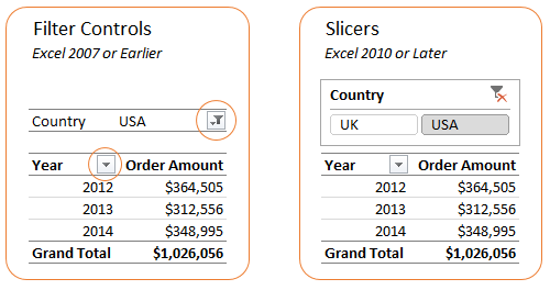
PivotTables are great at allowing you to easily filter the data using the built in filter controls, or if you have Excel 2010 or later you can use Slicers for a more polished and intuitive interface:

Now, while I love PivotTables I sometimes find they are too restrictive when it comes to charting the data.

For example, you can’t create a chart like this with a PivotTable:

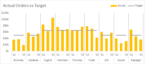
BTW, I teach you how to create charts like the one above in my Excel Dashboard course.

That’s when you need to call on Formulas to get the summarising job done, and the great news is we can link formulas to Data Validation lists so they’re interactive just like PivotTable filters or Slicers. Let’s look at an example.

Interactive SUMIFS Formula

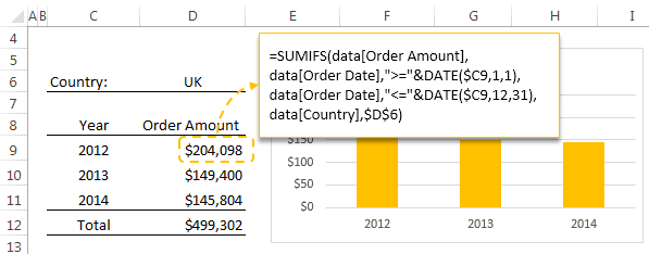
Below is my PivotTable looky-likey built using the SUMIFS function and a Data Validation list to control the country selection.

Looks just like the PivotTable, only nicer 🙂

Setting Up Interactive SUMIFS Formulas

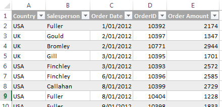
First let me introduce the data; below is a sample of it which is formatted in an Excel Table called ‘data’ (note: Since I’ve formatted my data in a Table I’ll be using Structured References in my formulas):

And the SUMIFS formula in cell D9 is:

Remember the syntax for SUMIFS is:

=SUMIFS(the range you want to sum,
range containing criteria 1, criteria 1,
range containing criteria 2, criteria 2,
range containing criteria 3, criteria 3…..)

Therefore the formula in cell D9 in English reads:

SUM the values in the Order Amount column IF,
the values in the Order date column are, greater than or equal to 1 Jan 2012 AND,
the values in the Order date column are, less than or equal to 31 Jan 2012 AND,
the values in the Country column are, equal to the country selected in cell D6.

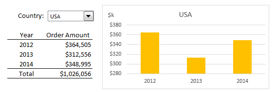
So, when the country selected in the data validation list in cell D6 changes, the SUMIFS formula automatically updates.

That is; by linking the third criteria to a cell containing a data validation list we have introduced a dynamic element which enables us to change the formula without having to edit it.

And when you use this data in a chart the chart becomes dynamic too (see example below).

Mix and Match

This technique isn’t limited to the SUMIFS function. Any of the …IF functions are ideal for dynamism e.g. SUMIF, COUNTIF, COUNTIFS, AVERAGEIF etc. and of course SUMPRODUCT.

You can also make any of the criteria (like dates) dynamic by simply linking the ‘criteria’ arguments to a cell containing a data validation list.

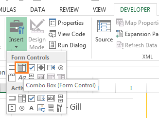
Combo Boxes

Combo boxes are an alternative to Data Validation lists.

You’ll find them on the Developer tab of the Ribbon:

The upside of a Combo Box is the drop down indicator is always visible, as you can see below:

The downside is they require an extra step since they return the position of the selected value in the list as opposed to the value itself (as seen in cell D33 below – i.e. USA is 2^nd in the list).

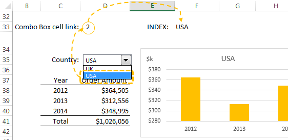
The solution is to use the INDEX function to lookup the cells containing the list and return the actual value, as can be seen in cell F33 above which contains this formula:

=INDEX(region[Regions],D33)

Where the INDEX funtion looks up the 'Regions' column in the table called 'Region', and returns the value in the row number based on the item selected in the Combo Box.

You can then reference the value in D33 in your SUMIFS formula, or insert the INDEX formula directly inside your SUMIFS like this:

=SUMIFS(data[Order Amount],
data[Order Date],">="&DATE($C38,1,1),
data[Order Date],"<="&DATE($C38,12,31),
data[Country],INDEX(region[Regions],$D$33)))

If you'd like to learn more techniques to make your Excel reports zing take a look at my Excel Dashboard course.