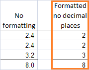
It’s common practice in Excel to format decimal places to get the desired rounding of numbers. But the problem with this approach is it can display totals that don’t appear to add up correctly.
Take the screen shot below that shows 2+2+3=8. That’s because the underlying numbers are actually 2.4+2.4+3.2.
 |
Excel ROUND Formulas
The solution is to use Excel’s ROUND, ROUNDUP or ROUNDDOWN functions.
- ROUND rounds a number to a specified number of digits
- ROUNDUP rounds a number up, away from zero
- ROUNDDOWN rounds a number down, towards zero
Let’s take the number 2.4 and round it to no decimal places as an example.
Using ROUNDUP you’ll get 3.
Using ROUNDDOWN you’ll get 2.
Using ROUND you’ll also get 2. ROUND will round down anything under 5, and round up anything 5 and over.
How to enter a ROUND formula
The ROUND, ROUNDUP, ROUNDDOWN functions can be applied to a cell, combined with other functions or even contain their own calculation.
Let’s take ROUND on its own first.
The Excel sytax is
=ROUND(number,num_digits)
In English it means:
=ROUND(cell reference (e.g. C2) or calculation (e.g. 5.3+2), the number of decimal places you want)
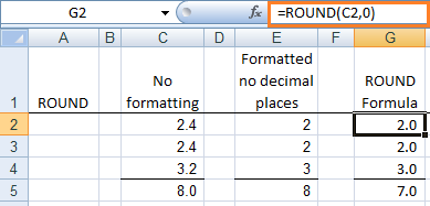
In the image below we can see ROUND in the formula bar as
=ROUND(C2,0)
Note: You can see that even though I’ve told Excel to round my number to zero decimal places in cell G2 it’s still displaying the number as 2.0. This is simply because the cell formatting is to one decimal place.
 |
Let’s say I wanted to round the number 2.489 to 2 decimal places. My formulas would read:
=ROUND(2.489,2) would give you 2.49
=ROUNDUP(2.489,2) would give you 2.49
=ROUNDDOWN(2.489,2) would give you 2.48
Ok, so that’s pretty easy. Let’s look at how we’d use a ROUND function with another funciton.
ROUND with another function
ROUND a SUM to no decimal places =ROUND(SUM(C1:C10),0)
You can see the ROUND formula is wrapped around the SUM formula.
ROUNDUP with IF =ROUNDUP(IF(C10>=450,C10*9%,""),0)
ROUNDDOWN with AVERAGE =ROUNDDOWN(AVERAGE(C1:C10),0)
You’re not limited to these examples above, ROUND can be used with almost any function.
ROUND to the nearest 5 cents
What say you priced products in 5 cent increments, but you found that when you marked up the cost price you often ended up with an amount that didn’t end in a 5 or a whole number. Take the example below where the selling price calculates at $9.96, but you have to price it at $9.95 or $10.00.
You can use the ROUND functions here too.
 |
By dividing the calculation by 5 cents (0.05) and rounding it to 0 decimal places, you can then multiply it by 5 cents (0.05) to get the correct amount.
If you wanted to round to the nearest 50 cents you would just replace the two instances of 0.05 with 0.50.
Alternatively you could use the CEILING or FLOOR functions to do this.
Enter your email address below to download the sample workbook.
Did you find this useful, or did it open a can of worms? Let us know by leaving a comment.
Share the knowledge with your friends and colleagues on Twitter, Facebook, Google+, LinkedIn etc.

Hi,
Can you help me with a formula? 🙂
For exemple:
I have the flowing prices to round them 48.99, 57.99, 66.99 —>49.99, 59.99, 69.99
And for 43.99, 52.99, 11.99 —-> 44.99, 54.99, 14.99
And for 40.99, 80.99, 60.99 —-> 39.99, 79.99, 59.99
Thank you!
Andy
Hi Andy,
You need to use the CEILING or FLOOR functions for this. If you’re still stuck, please post your question on our Excel forum where you can also upload a sample file and we can help you further.
This opened up a can with more worms…trying to round in the following formula, x.xx5 numbers are rounded down…=ROUND(PRODUCT(H30,12.5%),2)
Hi Sue,
Did you try =ROUND(PRODUCT(H30,12.5%),4)
Mynda
Hello,
How would I get excel to continue to round up the highest fractions in a column until it hits a specific number then round down the remain.
Example:
C1: 9.43, C2: 9.78, C3: 8.6
I want excel to round the highest fractions first until it equals 28. Then round the remain down.
So since C3 is the highest it rounds to 9, c2 is the second it rounds to 10, c1 is not needed to round up as we have hit our total so it rounds down.
Then I want to capture the fractions that it rounded up or down so they offset next month.
Example carryover:
C1= .43, c2=-.22, c3=-.4
Thank you,
Craig
Hi Craig,
Hard to follow your logic, something is missing. Can you provide an example file with a manual result filled in? Use our forum (create anew topic after sign in)
I’m trying to create a rounding formula that from $0 – $3 rounds to the nearest 5c increment, from $3.01 – $5 to the nearest 10c increment, from $5.01 – $10 the nearest 50c increment. from $10.01 – $20 the nearest $, from $20.01 – $50 the nearest $5 increment and above $50 the nearest $10 increment.
Is this possible?
Hi Manfred,
Try:
=CEILING(A1,INDEX({0.05,0.1,0.5,1,5,10},MATCH(A1,{0,3,5,10,20,50},1)))
Replace CEILING with FLOOR to see the results. CEILING will always roundup to the NEXT increment, FLOOR will round down to the next increment.
For example, if the value is 3.67, and the increment for this is 0.1, CEILING will return 3.7, FLOOR will return 3.6. The same results will be returned if the value is 3.62.
Thanks that’s awesome – works great!!!
you just saved hours of messing around … thanks for the post
You’re welcome, glad to help.
I search a formula to roundup & rounddown using if condition,
(if a1=>.50 then roundup to Rs. 1 else rounddown to Rs. 1)
Kindly help
Thanks
Try this one:
=IF(A1>=0.5,ROUNDUP(…),ROUNDDOWN(…))
I guess that you do not mean A1>=0.50, do you mean just the decimal part?
If so, simply use ROUND(A1,0). By default, if the decimal part is above or equal to 0.5, a roundup will be applied, otherwise a rounddown is applied.
$5,151.66
$24,490.51
$106.35
$4,931.73
$3,202.29
$3,501.54
$2,919.04
$545.37
$151.51
The above numbers have to total 45K, when rounded to a whole number they come to a value of 45,001. The general formula for rounding works except on the 24,490.51 this gets rounded to 24,491 which makes all the numbers added up to 45,001. What I need to to be able to round the above numbers to a whole number that will return 45K even. I have been trying to work on a roundup/round down if statement to try and make this work. Any help which be much appreciated
Hi Paulette,
Rounding 24,490.51 to 24,491 is correct.
Rather than use the ROUND function, just decrease the displayed number of decimals for each of your numbers. This will display them as rounded, but will add up to 45,000.
Regards
Phil
Hi Every one
I’d like to thank every one for sharing the knowledge
** My Question is :
I Want a functions that round numbers to nearest 45 or 95 , For Example :
A (Original) B (Manually Entered)
1- 370 395
2- 3043 3045
3- 99 145
Best Regards,
This post explains how to round to the nearest 45 or 95.
10000 15000 20000
i want round off the three value in excel in what will the single value for these three value
Hi Ashok,
Not sure what you mean. Sounds like you want to get the average of these three numbers? Which would be (10000 + 15000 + 20000) / 3 = 15000
Regards
Phil
How would I make this formula roundup
=(H51/(1-K45))+D50+(C49*(H51/(1-K45)))
Hi Matt,
You haven’t said how many decimal places you want to round up to, but assuming zero it would be:
Mynda
Hi there,
I am trying to project the number of monthly sales per phase of product released. We release product for sale in phases, and I’m assuming a total of 4 sales a month among all phase releases. We currently have 8 phases available for sale. I created a formula to count the number of phases that are available for sale, and divide that number into the number of projected sales per month. As you can imagine, 4/8 equals .5 sales per phase per month, however showing half a sale isn’t realistic since sales need to be in whole numbers – so to address this I used the round function but this is now bringing me to 1 sale per phase per month for a total of 8 sales – double the realistic monthly projection. How can I get 4 out of the 8 phases to show 1 sale and the rest to show 0 sales, for a total of 4 sales per month? Is there a way to work from top to bottom – populating the earlier phase releases with the sales first until they run out of product and then working it’s way down to later phase releases? This is my current formula. Help much appreciated, thank you.
(ROUND((INDEX(Seasonality!$I$6:$T$42, MATCH(Template!$C$2, Seasonality!$H$6:$H$42, 1), MATCH(MONTH(Template!I$5),Seasonality!$I$3:$T$3, 0)))/COUNTIFS($F$6:$F$363, “=Remaining to Sell”, H6:H363, “>0”),0)
The first part of the formula is plugging the avg sales rate into my seasonality table which takes into account busy/slow seasons. For purposes here, the month in question has a projected sales rate of 4 as mentioned above. The second part is counting phases with product remaining to sell.
Hi Rachel,
Can you please upload a sample file on our forum with a manual set of expected results? It will be easier to work on a file to provide a customized solution, rather than a generic answer.
You can create a new topic after sign-in, to upload the file and details.
Thanks
Great Explanation. I just found your website and I think it is great. I am trying to learn VBA but some of the things I want to do can be done without VBA coding. I found some of the answers I needed in your excellent website. Thanks
Lloyd
Thanks, Lloyd! Glad we could help 🙂
im am rounding up at the moment but would like to round up and down in same cell if the sum is higher or lower than 1000.
this is the formula i am using currently
=ROUNDUP(SUM(E17-D17)/480,0)
Hi Brian,
You need to use an IF function too
This assumes:
– The number being rounded is in A1. Replace A1 with your SUM() or other calculation
– You are rounding to 1 decimal place
– Numbers greater than or equal to 1000 are rounded up. Your original qs did not specify what to do when the number being rounded was equal to 1000
Cheers
Phil
10>round up to the nearst whole number
100>roundup to the nearst multiple of 5
1000> roundup to the nearst multiple of 10
10000>roundup multiple of 50
50000>roundup Multiple of 100
100000> roundup multiple of 1000
100000<roundup multiple of 10000
Excel Formula:
Hi Muhammad,
You’ll need to use the CEILING function for this
Regards
Phil
thanks
Hello,
I am trying to do a rounding up function. i am taking a product length such as a 11′-6″ and trying to round it up to 12′. the biggest issue i am having is it needs to be X by a price for
Example 1; 11′-6″ x $3.76 should = $43.24.
Example 2; 11′-5″ x $3.76 should = $41.36.
can anyone help me on this?
Thanks
Chris
11′-6″ is a text, not a number.
You have to use vba to convert it to decimal inches, to perform calculations on it: try the code from this page: https://social.msdn.microsoft.com/Forums/office/en-US/323edef9-be0d-4f1b-a383-fec5a44be93a/excel-2010-feetinches?forum=olbasics
I seem to be still having a hard time. the link supplied doesn’t seem to make sense the code it asked me to wright seems to not work.
Hi Chris,
I use that code frequently and works. I copied the code from the link in a workbook for you, and used it for a few conversions, works right out of the box, not sure why you are having trouble using it, make sure you type the apostrophy and double quote from keyboard, if you paste them from browser they are different.
Here is the file from our OneDrive you can test, all set.
Cheers,
Catalin
Penny says
Hi Andy,
HELP!!
Trying to Creating a spreadsheet for a point system for golf.
I’m try to divide a number in a cell then round down, the number is odd (points need to pull for each 9 hole.
Example: 13/2 = 6.5 in 1cell and 7 in the next cell. Then I putting in points for what they pulled on 1st 9 holes. The answer needs to minus 6 only not the 6.5.
Thank you
Hi Penny,
So you want to round 6.5 down to 6?
=ROUNDDOWN(6.5,0)
or generally, if you have a value in A1, the formula would be
=ROUNDDOWN(A1,0)
regards
Phil
Hi there
I’m putting together a golf handicap spreadsheet where we have 0.25 shot adjustments. The problem is we round down if the handicap is over 28 and round up if under 28.
For example 33.75 = 33 and 19.25 =20.
Is this possible in a formula?
Hi Andy,
Try this formula:
=IF(A1>28,FLOOR(A1,0.25),CEILING(A1,0.25))
Hi, How do i rounding number such as
0.0 to 0.0
0.1 to 0.0
0.2 to 0.0
0.3 to 0.0
0.4 to 0.0
0.5 to 0.5
0.6 to 1.0
0.7 to 1.0
0.8 to 1.0
0.9 to 1.0
1.0 to 1.0
Apply for negative value also.
Can anyone help? Thanks!
Hi Ace,
Try this formula:
=IF(A1-INT(A1)<0.5,FLOOR(A1,0.5),CEILING(A1,0.5))
Hi Catalin,
The formula is working, thank you for your help!
You’re wellcome 🙂
I am using this formula
=COUNTA(C2:C397)/1965*100&” authentication failure”
The value returned is:
20.1526717557252 authentication failure
How can I round the number in my formula?
Hi Bruce,
This should work, it’s the usual round function:
=Round(COUNTA(C2:C397)/1965*100,2)&” authentication failure”
Hello I am creating a spreadsheet with 2 separate formulas to conduct accountability of bottles used to the nearest .25 of the bottle. Formula #1 is {=((E5-F4)*(H4*2))/100}. I have the following answers using this formula [1.19; 1.03; 4.36]. The answers I am looking for is “1.25; 1.00; 4.50”. Thank you.
Hi John,
It’s difficult to visualise how this formula {=((E5-F4)*(H4*2))/100} is returning 3 results: [1.19; 1.03; 4.36]
Can you please post your question on our Excel Forum and upload a sample Excel file so we can help you further.
Mynda
Roundup/rounddown etc work fine for rounding to xxxx decimal. but how to round absolute figure (no decimsls)? for example how to round 123456 to nearest tens/hundreds/ thousands etc? Do this,…..round(123456,-1) or round(123456,-2) or -3 or -4……[email protected]
Hi Anantha,
To round to the nearest integer, no decimal places, use 0 : ROUND(123.12,0)
If you don’t want to round, you can remove decimals with INT(123.12)
I am working on a percentage increase in cost, so my equation is:
=(C2*4%)+C2
My problem is how do I write this equation, so it rounds down if under $.50 and rounds up if over $.50?
Hi Joyce,
Try this:
Mynda
I think you may be the one to help me figure out a rounding formula for my upcoming price increase!
I need to perform the following rounding schedule and can’t figure out the formula.
Thanks in advance for your help!!!
$0.01-$0.99=Actual
$1.00-$5.99=Round up to the nearest $0.05
$6.00-$9.99=Round up to the nearest $0.10
$10.00-$19.99=Round up to the nearest $0.25
$20.00-$49.99=Round up to the nearest $0.50
$50.00-up=Round up to the nearest $1.00
Hi,
Try this one (the price should be in A1):
=CEILING(A1,IF(A1<1,A1,INDEX({0.05,0.1,0.25,0.5,1},MATCH(A1,{1,6,10,20,50},1))))
Sir,
suppose i have the values like 2.2 3.1.3.2, 4.2
the round function gives values 2, 3, 3 and 4 respectively but if we sumup these values the value shall again be 13 instead of 12, how i can get the value 12
Hi Suhail,
If you wrap your SUM in the INT function it will drop the decimal places off the result, is that what you want?
Mynda
Great help……to gain an understanding of formulas
Hi Jeff,
Glad to hear you like our tutorials 🙂
Cheers
Catalin
Help!! Need to resolve a rounding error. If cell T3 is rounded and O3 is not, but a whole number … How do I adjust the formula to account for a rounding issue? Basically if its less than a dollar variance the formula should not reflect the “check” error.
Formula I’m currently using is: =IF(T3>O3,”check”,”-“)
Hi Jennifer,
You can try this formula:
Mynda
It opened a can of worms coz when my problem was solved i jumped too hard and it opened a can of worms.
Rounding on a spreadsheet. New Sales taxes rule is now requiring my spreadsheet to round up or down. If an amount that ends .49 cents or lower, then round amount down to the previous dollar, for the amount is .50 cents or higher, then round amount up to the next dollar.
Please help me with the rounding formula.
Here are a couple example of some sums on my spreadsheet
=SUM(E9:E10)
=SUM(K9*0.03)
Thanks for the help.
Hi Tammy,
You can use teh CEILING and FLOOR functions for this:
https://www.myonlinetraininghub.com/excel-ceiling-and-floor-functions
Mynda
Know one seems to understand. I want the answer to a formal to always Round up to a whole number.
Hi John,
Have you tried =ROUNDUP(A1,0) ?
Catalin
Hey Mynda,
Bit of a strange question here, but if anyone an answer it you can!
I have designed a stock taking sheet for my bar that doubles up as an order sheet for our suppliers.
Obviously stocktaking requires accuracy to .1 of a bottle, whereas an order has to be rounded to the nearest whole bottle. So far, so easy right? SO the formula goes like this: =ROUND(C14-D14) where C14 is par stock level and D14 is current stock level.
However where it gets complicated is for tope shelf/high value bottles which are sold infrequently we don’t want too much of hanging around in stock. As present, as long as the in-stock value is 0.5 or lower, there will be a command to order another bottle (rounding up from 0.5). I wonder is there any way to make it so that the formula will round DOWN from a value as high as say 0.7 but then round UP fro values of 0.8 or higher?
Thanks in advance for putting your knowledge and abilities to this.
All best,
Edmund
Hi Edmund,
You can check the remainder with MOD function, then apply the appropriate roundup or rounddown:
=IF(MOD(A1,1)>0.7,ROUNDUP(A1,0),ROUNDDOWN(A1,0))
Catalin
Plz tell me the formula when
E.g.. (E6+F6)×113% in round figure
Hi Harry,
I assume you want it rounded to no decimal places. If so:
=ROUND((E6+F6)*113%,0)
Replace ROUND with ROUNDUP or ROUNDDOWN if required.
Mynda
If I only want to round a vlaue if it is above 50,000.00 so 28,560.00 would be 0.00 but 504,288.00 would be 504,200.00 what =round formula should I use?
Hi Mark,
You should try this:
=IF(A1<50000,0,ROUNDDOWN(A1,-2))
Catalin
Hi Mynda,
I’m trying to round numbers to the nearest dollar, but I need to truncate the results so that I’m left only with an integer value. So if I’m adding three rounded numbers together, I don’t want the decimal amounts included in the total, just the rounded integer value.
To better illustrate, take the example below:
Amount 1 – $1.45 – rounded down, it would be $1.00
Amount 2 – $1.60 – rounded up, it would be $2.00
Amount 3 – $1.48 – rounded down, it would be $1.00
The exact total is $4.53. If I add the rounded values, I’ll get $5.00. However, I want the decimals removed once they have been rounded. So the answer I’m looking for is $4, the sum of the integers only resulting from the rounding action. Can you please help?
Thanks,
Sean
Hi Sean,
If you use Round on the sum of those 3 amounts, you will get 5. Use =Round($1.45,0)+Round($1.60,0)+Round($1.48,0), the result will be 4.
Cheers,
Catalin
Thanks Mynda,
If I was to add the rounddown to nearest 5 function to this formula =D13-(D13*E10) it’d look like:
=rounddown((D13-(D13*E10)/0.05,0)*0.05 ?
best,Paul
No, like this:
totally stuck on how to round the following formula down to nearest 5, any suggestions?
=SUM((D$2*C13)*52)/12
Every combination I do it says I’ve added too few arguments… sorry guys!
Hi Paul,
You can use this formula:
No need for SUM unless you want to SUM a range of cells.
Kind regards,
Mynda
There is an easier method to ROUND to the nearest 5 cents =MROUND(12365.042, 0.05) you get 12365.05
Thanks, Nelson. Great tip.
They (MS) really should have named that ROUNDM so it doesn’t get overlooked!
Mynda
YES!!!!!! THANK YOU VERY MUCH MYNDA, I HAVE FOUND A SOLUTION THAT HAS BEEN UNKNOWN TO ME AND A LOT OF MY CO-TEACHERS HERE IN YOUR SITE . NOW WE CAN USE THE FORMULA TO OUR HEARTS CONTENT, ELIMINATING UNNECESSARY LONG CUT. KUDOS TO YOU….. GOD BLESS
You’re welcome, Gary 🙂
Thank you for this tutorial – just what I needed 🙂 I’m sure i’ll be back for more help !
Jane
You’re welcome, Jane. Be great to see you back here again sometime.
Help! I need the formula to multiply a cell by 60% then roundup to the nearest $.25. I’ve entered it several ways but it rounds down 5.30 to 5.25.
Hi Ellie,
Use this
Catalin
Very helpful, thank you. Having spent a good couple of hours trying to complete one function, your site helped me do it in a matter of minutes!
Thanks, Ann. Nice of you to take the time to leave a message. I’m glad I could help 🙂
Hi
My Dear honest teacher Mynda I hope you will doing well with your noble family.
Thanks for your nice Information you share with all people i appreciate you.
you know i am trainer of office program bot i am not professional trainer bot i hope to be a good teacher in the future if you help me.
please i hope you will accept my request i will waiting for your good news.
Thanks for again have a good time with your noble family.
Hi Hafizullah,
Thanks for your kind words. You can find a list of free tutorials on Excel Formulas here, plus have a read through our blog for other tutorials.
All the best.
Mynda.
Hi!
I have the following situation:
I have a column with cells like this one
=5.83/11
= 7.88/11 and so on
I would like to add Round formula with copy-paste but keeping the original numbers, without doing it manually for each cell. Is it possible?
I’ve made one modification manually but when I use Paste Special – Formula it changes also the numbers (if I copy from the cell with 5.83 in the cell with 7.88, 7.88 changes in 5.83.
Thank you very much!
Hi Lala,
Honestly, I don’t quite get what you mean here.
Why don’t you send your file and label the things that happened.
Send it here: HELP DESK
Cheers,
CarloE
Mynda
Thank you for making this understandable and easy to follow. I am writing you this down in the jungle of DR Congo and there is no Excel help within a distance of at least 800kms, and that will not be in English! I will come back to you for more Excel related questions – if you do not mind.
Kind regards
Abraham
Thanks for your kind words, Abraham 🙂
I would line to round average that IF 0.50 round down and IF 0.51 round up
Hi Vicktor,
You can use this formula:
Kind regards,
Mynda.
i want to set round function at .99 ..like if i have no.>=50.99 then it will return 51 else it will return 50. plz tell me how it is possible…?
Hi Lalit,
=IF((RIGHT(A1,2)=”99″),ROUND(A1,0),ROUNDDOWN(A1,0))
Where A1 contains your value 50.99
Kind regards,
Mynda.
I entered a bunch of UPC numbers into an excel spread sheet for hundreds of my products. I saved it and closed it. When I opened it back up all the numbers with more than 11 digits changed to only keeping the first three numbers and then rounding down to all zeros for the rest of the numbers! This was hours of work. Can I get my original numbers back or do I have to enter them all again!? Help! 🙂
Thanks.
Hi Gary,
Have you tried to change the formatting of the cell to ‘Number’?
To do this press CTRL+1 > on the ‘Number’ tab select ‘Number’ from the category list.
Does this fix the problem?
If not send me your workbook by logging a ticket on the help desk and I’ll take a look.
Kind regards,
Mynda.
Thank you! This was a great help!
does anyone know if you can apply the round function to a column of numbers such that you would not need to enter the formula in another column?
Hi Sean,
The only way you can apply any sort of rounding to an existing column of numbers (that are not formulas) is to use formatting, but as I mentioned above, this isn’t true rounding.
The other option you have is to insert the ROUND formula in another column, then Copy and Paste Special > Values back to your original column, then you can delete the column with the ROUND formula as it’s no longer required.
Alternatively, if the column that you want to round contains a formula you can wrap the ROUND formula around your existing formula.
For example;
=ROUND(A1/B1,2)
=ROUND(SUM(G11:G14),2)
There are more examples in the tutorial above.
I hope one of those solutions is suitable.
Regards,
Mynda.
Had found a few examples on the internet – but this is the only one that really made it clear enough to add it to my word doc. Very easy to use – really fantastic.
Thanks Rick. Glad I could help.
thanks, I appreciate the time you took to write this, its all very clear with the different colours and images 🙂
J