Excel VSTACK and HSTACK Functions

Excel VSTACK and HSTACK functions are just two of a raft of new text manipulation functions available to Microsoft 365 users.

I wrote about text splitting functions TEXTSPLIT, TEXTBEFORE and TEXTAFTER a while back.

The new VSTACK and HSTACK functions work to combine arrays arranged vertically (VSTACK) or horizontally (HSTACK) into a new single array.

Watch the Excel VSTACK and HSTACK Functions Video

Download Workbook

VSTACK Function Syntax

Syntax: =VSTACK(array1,[array2],...)

array     The arrays (cell ranges) you want to append.

HSTACK Function Syntax

Syntax: =HSTACK(array1,[array2],...)

array     The arrays (cell ranges) you want to append.

The syntax is fairly straight forward, but there are some clever techniques we can use to enable stacking data from multiple sheets, sorting, specify headers, filters, handle errors and more.

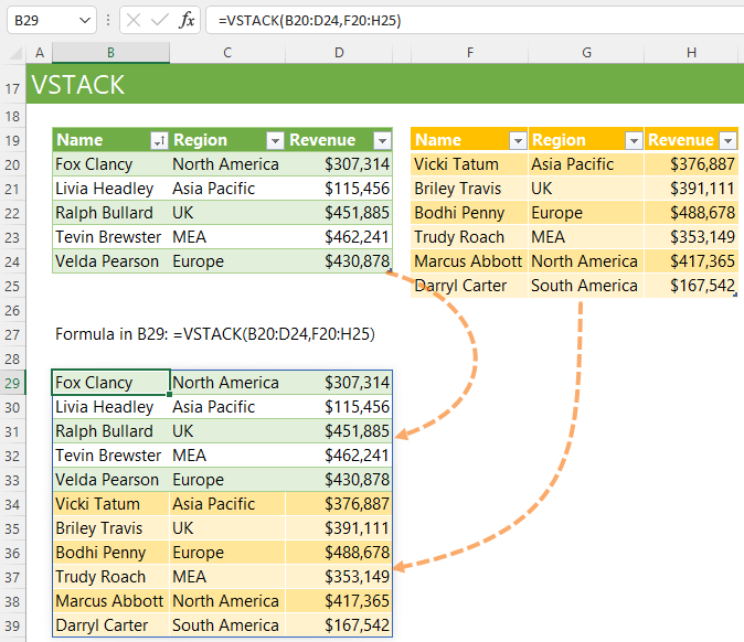
Example 1: VSTACK Two Arrays

In its simplest form, VSTACK combines multiple arrays of the same number of columns:

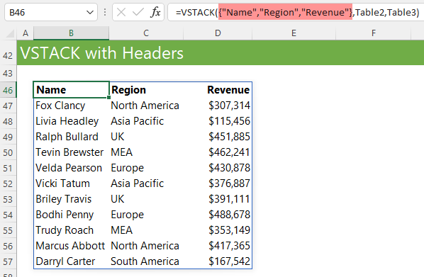
Example 2: VSTACK with Headers

Column headers can be added to the stack by entering them in the first array argument as shown below, or referencing an array that contains the labels:

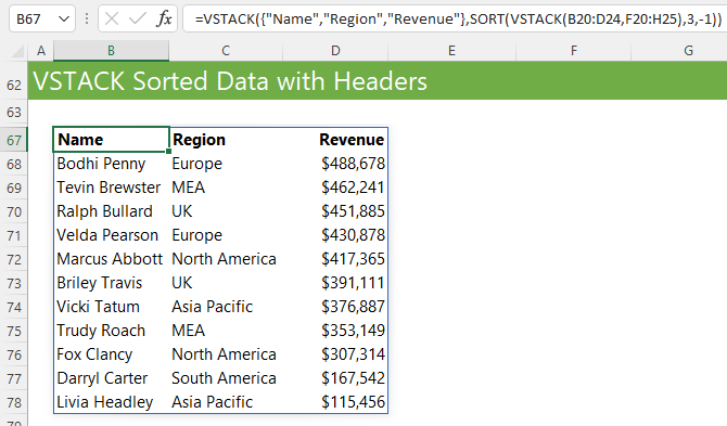
Example 3: VSTACK Sorted Data with Headers

We can nest VSTACK functions inside one another to enable sorting of the data using the SORT function separate to the headers:

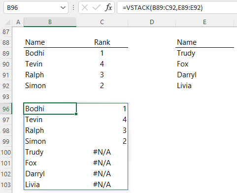
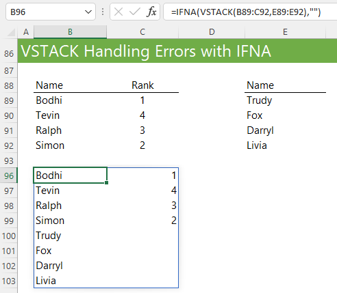
Example 4: VSTACK Handling Errors with IFNA

If the arrays being stacked are different sizes, VSTACK will return #N/A! errors in place of the missing data:

Wrapping the formula in IFNA enables you to specify something else in place of the errors. In the example below I’ve used two double quotes so the cell appears empty, but you could also enter some text in here like, “Missing Data”:

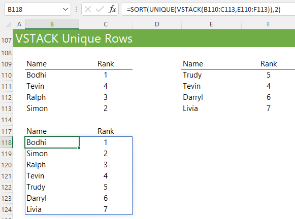
Example 5: VSTACK Unique Rows Only

Omitting duplicates from the final array is easy with the UNIQUE function:

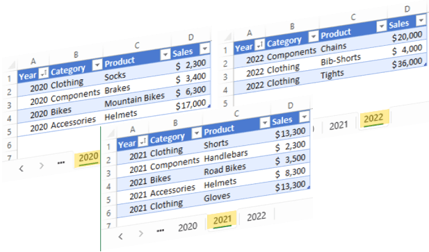
Example 6: VSTACK 3D Range

You can stack data spread across multiple sheets. In the images below you can see I have data containing the same number of columns, but a different number of rows on 3 separate sheets:

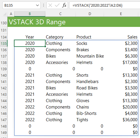
I can use VSTACK with a 3D reference to stack them all into one array. Now, because I need to allow for the table containing the largest number of rows in my range it results in zeros being returned for the tables that don’t contain data on rows 5 and 6. We’ll look at hiding these blanks in the next example.

Tip: If your data is formatted in an Excel Table, you could simply reference the 3 table names separately e.g.:

=VSTACK(Sales_20,Sales_21,Sales_22)

If the data grows, the formula will automatically include the new data.

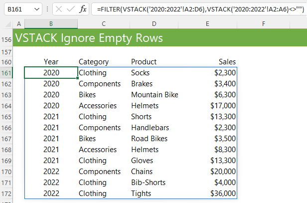
Example 7: VSTACK Ignore Empty Rows

The previous example contained some empty rows which resulted in zeros throughout the final array. We can use the FILTER function to exclude those rows from our stack:

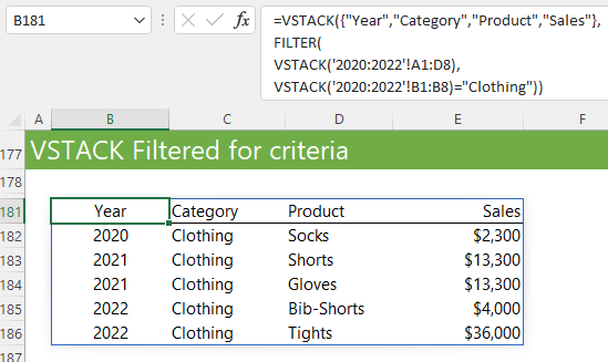
Example 8: VSTACK Filtered for Criteria

Similar, to the previous example, we can filter for specific criteria. In the example below I’ve used VSTACK three times:

1. For the headings
2. For the range being stacked
3. For the column containing my criteria used by filter

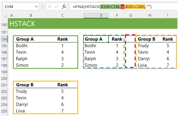
Example 9: HSTACK

HSTACK is the horizontal stacking equivalent of VSTACK, so we’ll just look at one scenario for completeness. The example below shows how we can combine two vertically arranged sets of data into a horizontal array. Notice the use of the two double quotes in the middle HSTACK argument to allow for a blank column between the two groups of data:

VSTACK and HSTACK 3D Reference Limitations

One of the advantages of the ‘STACK’ functions is they can be used to make 3D references work with any function that doesn’t have support, except those functions that require a range as an input.

Remember, a 3D reference is one that references multiple sheets, like we looked at in example 6:

Here we used VSTACK to append it together into one array with the following formula:

=VSTACK('2020:2022'!A2:D6)

Another common 3D formula is to sum the data on those three sheets like so:

=SUM('2020:2022'!D2:D6)

We can do this because the SUM function supports 3D references. Here’s list of all functions that support 3D references.

However, what if you wanted to sum the data for the Clothing category on those three sheets? You might try to write this SUMIF formula:

=SUMIF('2020:2022'!D2:D6,'2020:2022'!B2:B6="Clothing",'2020:2022'!D2:D6)

And you’d find it returns the #VALUE! error because the SUMIF function requires a range as the first argument. And because of this you can’t use VSTACK for the range argument because VSTACK returns an array, not a range. Instead, you could use one of the following formulas:

=SUMPRODUCT(--(VSTACK('2020:2022'!B2:B6)="Clothing")*VSTACK('2020:2022'!D2:D6))

Or

=SUM(--(VSTACK('2020:2022'!B2:B6)="Clothing")*(VSTACK('2020:2022'!D2:D6)))

VLOOKUP and XLOOKUP on the other hand do accept VSTACK in the array arguments. For example, say I want to lookup the sales for socks, I can write:

=VLOOKUP("Socks",VSTACK('2020:2022'!C2:D6),2,0)

Or

=XLOOKUP("Socks",VSTACK('2020:2022'!C2:C6),VSTACK('2020:2022'!D2:D6))