A little while ago I showed you how to do a lookup to the left using the INDEX and MATCH functions.
In this Excel tutorial I’m going to show you how you can do a lookup to the left with a VLOOKUP formula together with the CHOOSE function as an alternative.
Let’s look at our data:
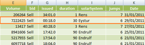
In this example we want to look up the Volume in column E for the date 29/01/2011 in column K. As we know, a VLOOKUP cannot go left, but with the help of the CHOOSE function we can trick it into going left.
CHOOSE Function
First of all let’s understand how the CHOOSE function works:
This is the syntax in Excel:
=CHOOSE(index_num, value1, value2, value3…..up to 254 values)
The syntax is not very useful as usual! To translate it into English:
=CHOOSE(value number 3 where, value 1 = A, value 2 = B, value 3 = C)
The result is C
Now we can get creative by specifying more than one index number with the help of curly brackets { }, and instead of specifying the values (like we did above with A, B and C) we can refer to a range of cells like this:
=CHOOSE({1,2},$K$2:$K$207,$E$2:$E$207)
In English this formula reads:
= ({column 1 is K , and column 2 is E})
Effectively switching the positions of column E and K so that the VLOOKUP will think column K is to the left of column E. Clever, huh?
VLOOKUP to the Left
Now, on its own, like the example above, CHOOSE is not much use but when you use it in a VLOOKUP it enables us to trick Excel into returning the value to the left of our lookup column.
Our formula to look up date 29th January 2011 in column K and return the value in column E (column number 2) is:
=VLOOKUP(DATE(2011,1,29),CHOOSE({1,2},$K$2:$K$207,$E$2:$E$207),2,0)
Translated:
=VLOOKUP(find 29/01/2011 in column K and return the value in column E)
Result 7,222,425
NOTE: When you want to reference a date in a formula you need to tell Excel it is a date using the DATE function, alternatively you can use the date’s serial value. However, I find the DATE function more intuitive and easier to follow when I revisit a formula later on. Alternatively you could reference another cell that contains the date in the correct date format.
TIP: We can make this formula a little easier to use by changing the cell range references to full column references. This will work in this instance because there is no other data in our columns other than that which is in our table.
With full column references our formula looks like this:
=VLOOKUP(DATE(2011,1,29),CHOOSE({1,2},K:K,E:E),2,0)
Enter your email address below to download the sample workbook.
In some ways I think using the CHOOSE function to trick your VLOOKUP to look left is easier than the INDEX and MATCH functions , especially if you're more familiar with VLOOKUP.
What do you think? Do you have a preference or do you just rearrange your columns so you never have to lookup to the left? Let me know in the comments below.

Forgot to mention. INDEX() can also put non-contiguous areas together using an array constant in the “Area” parameter (4th parameter, the one no one ever uses).
So you then have a contiguous internal-to-the-formula table for something like VLOOKUP() to use. So using it with VLOOKUP() can give you one of the major advantages of XLOOKUP() and INDEX/MATCH (being able to specify mostly unrelated columns) but still have the family-friendly function instead of a prickly one.
And if you don’t have the newer functions…
It won’t cross pages though. In the sense of the ranges being put together being on different worksheets. Even in the group listing, it insists upon all of them being the same page.
It’s a useful start in being able to put non-contiguous ranges into a single column, rather than one column for each range, as used above.
Rather than use CHOOSE(), which I dislike for a number of reasons and regard as quirky due to some of its returns, I use INDEX():
=VLOOKUP( M1, INDEX( A1:F100, ROW(1:100), {2,1}), 2, FALSE)
which looks at the range A1:F100, includes all the rows in the lookup, but only uses columns 2 and 1 (columns B and A), letting you choose the columns to use better than CHOOSE() does, and it uses those columns in the order you have specified. So like in the example, the columns’ order has changed from the “natural” columns A then B, to columns B then A.
I originally did this to “look left” just as INDEX/MATCH famously does, since the column order is reversed and VLOOKUP() looks right… but to a column that is left of the lookup column in the real range. Just not in the internal virtual range!
It also only looks at the two columns, so should be as fast as INDEX/MATCH in that respect, though I never bought the idea VLOOKUP() really places all 8,000 columns you have in your table when working anyway.
Using INDEX() like this has been possible in EVERY place I have been told to use CHOOSE().
Notes:
1. Since you are giving INDEX() an array constant for the columns, either directly, or perhaps with SEQUENCE() or by using a range instead, you must ignore all the explanations about how it does not need the row/s specified. It does. And… usually… you want them all so the usual ways of doing that need using: ROW(1:x) style, SEQUENCE() style, a range with entered values style, and more complex styles. Row is old school, but lets you easily use something like ROW(23:466) which is a little more complicated with SEQUENCE(). Whatever works for you.
2. In MOST, but not all, though the rhyme and reason escape me presently, INDEX() does not like array constants for both rows and columns, nor for one with a range for the other. But MOST of the time, it will take SEQUENCE() for one and whatever for the other, or SEQUENCE() for both. That last is nice though you have to remember to do something like SEQUENCE(1,2,2,-1) to get {2,1}, for example.
3. You can still use an array constant, or equivalent, in VLOOKUP() itself, for example the lookup parameter or the output column parameter. Using INDEX() to create an internal virtual table does not affect that.
4. IF YOU WISH, you can even transpose the table using INDEX(), performing a HORIZONTAL lookup with VLOOKUP(). (And vice-versa for HLOOKUP()…) If you EVER had any reason at all to do that with HLOOKUP() handy. Not to mention XLOOKUP(), INDEX/MATCH, and FILTER() lying about ready to use.)
Anyway, it’s a robust solution that fits a million needs.
Hi
First of all, I want to say thank you so much you for making available easy online data and providing such source to us. It’s really so easy to understand. One more time i have to say thank you.
I really appreciate that help
I owe you too much
Thank you
Our pleasure, Mahmoud!
I have used this formula to extract data from one work sheet to another to create a work schedule.
=VLOOKUP(B9,CHOOSE({1,2},’Desilt -AMP 7 Y1′!$Q$4:$Q$306,’Desilt -AMP 7 Y1′!$E$4:$E$306),2,0)
The Q column from the data source will remain blank and only be allocated a number once the work is scheduled, but does contain data in the E column. I wish to copy the formula in to several rows on sheet one and for the rows on this sheet to be populated once the job number is entered (manually by another party) into the B column (as long as columns B & Q match). By using this formula, with the Q column blank, it finds the first empty cell and returns the data from column E. Is there any way this formula can be adapted to leave the rows in the first sheet blank until the number is entered in the B column? I have tried the “” at the end of the formula, but this just returns an error.
Thanks
Hi Iwan,
Have you tried to wrap your formula into IFERROR function?
=IFERROR(your formula,””)
Thanks Catalin,
Worked a treat.
Regards,
Iwan
Question: Do the VLOOKUP-CHOOSE and the INDEX-MATCH combinations work when the lookup area is found in a different workbook?
You mean that INDEX range is in a workbook, and MATCH lookup range is in another workbook?
Will work only if the item row coresponds exactly between the 2 books, otherwise you will get wrong results.
First of all, I want to thank you for making available easy online data and providing such source to us. It’s really very easy to understand. Once again thank you.
You’re welcome, Kajal 🙂
Hello,
creating a custom range is very interesting and I can think of various contexts in which it would be helpful.
Is there a way to make this custom range dynamic? I.e. could you have something along these lines:
CHOOSE({A7,B7},$A$2:$A$4,$B$2:$B$4,$C$2:$C$4,$D$2:$D$4),
where if the values of A7 and B7 are 4 and 2 respectively
we would get a range containing $D$2:$D$4 in column 1 and $B$2:$B$4 in column 2?
Salut Radu,
A constants array must contain only constants, {A7,B7} is not a valid constants array, excel will reject the formula.
However, if you create a defined name and use this formula in the RefersTo range:
=CHOOSE(Sheet1!$A$7:$B$7,$A$2:$A$4,$B$2:$B$4,$C$2:$C$4,$D$2:$D$4)
you will get a range containing those 2 ranges indicated in A7 and B7.
Cheers,
Catalin
Salut Catalin,
many thanks, I shall try this out.
It may not be quite as flexible as what I was looking for but can certainly be useful.
All the best
Radu
You’re welcome.
You can also create a new topic on our forum with a sample file and a detailed description of what you’re trying to achieve, there can be more than one solution to any problem, I’m sure we can help you find a good solution here.
Salutari,
Catalin
If your cells for Choosing (A7, B7) are contiguous and linear (so A7:B7 but not A7:B8), you can specify a range using them:
=CHOOSE( A7:B7, $A$2:$A$4,$B$2:$B$4,$C$2:$C$4,$D$2:$D$4)
Also, to get the full data set, if your data are vertical, the range must be horizontal (like in your example and the formula above). If your data are horizontal, the range must be vertical.
If you cross over, horizontal data and range, you get an odd result. Not unique to CHOOSE(), but I consider it to be a major defect in working with CHOOSE().
By the way, the odd result is, using the 4 and 2 from your example, first cell in the column 4 is returned, second cell in column 2 is returned, and you get two N/A errors since it tries to return the third cell in your third column choice and the fourth cell in your fourth column choice… but you only specified the first two so it has no idea what to return for the last two and gives the error.
I’ll post a comment with INDEX() instead of CHOOSE().
Hi Roy, thanks for your insights! I’m interested to understand more about this cross over of horizontal data and ranges with odd results. I can’t visualise what you meant. It’d be great if you can email us with an example file so we can learn more. Mynda
This is very interesting and very clever indeed. I love nested functions since they show the hidden power of Excel. Thanks a lot.
Thanks, Hassan! Glad you enjoyed it 🙂
hello ,
I have one query that if i have some(50) different material with different rates and i give someone so i want to make his ledger in another sheet with add metrial name with qty and show his amount in last coloumn. Please guide.
thanks
Hi Ajay,
Try to prepare a sample file with details on our forum, create a new topic after sign-in.
Soy de Colombia no se ingles pero su pagina es increíble, los ejemplos y la explicación son muy útiles..gracias
De nada, me alegro de que haya sido útil.
Thank you very much. Very useful, easier and takes fewer memory resources to calculate compared to Index & Match combination.
Glad it was useful, Mohamed.
This is the first time I’ve seen CHOOSE used like this. Pretty cool…I have yet to try it. Any idea of how the calculation intensity compares with the INDEX/MATCH method? I often work with very large spreadsheets.
Hi James,
I’ve not tested the VLOOKUP and CHOOSE formula for performance, but I’d go with INDEX & MATCH every time. And to make it more efficient you can sort your ‘lookup’ data.
Mynda
not new 2 me, but I like the way you present/explain it
Thanks, Bruno 🙂
This is amazing! I learned something new today
In this example,how can we solve if lookup value has array of values like {date1,date2,date2}
Hi Prasanth,
Please post your question and a sample Excel file on our forum so we can see what you mean in the context of Excel.
Thanks,
Mynda
I have data like this:
Month Salesman Region Product Customers Net Sales Profit / Loss
Jan-07 Joseph North FastCar 8 1,592 563
Jan-07 Joseph North RapidZoo 8 1,088 397
Jan-07 Joseph West SuperGlue 8 1,680 753
Jan-07 Joseph West FastCar 9 2,133 923
Jan-07 Joseph West RapidZoo 10 1,610 579
Jan-07 Joseph Middle SuperGlue 10 1,540 570
Jan-07 Joseph Middle FastCar 7 1,316 428
Jan-07 Joseph Middle RapidZoo 7 1,799 709
Jan-07 Lawrence North SuperGlue 8 1,624 621
Jan-07 Lawrence North FastCar 6 726 236
Jan-07 Lawrence North RapidZoo 9 2,277 966
Jan-07 Lawrence West SuperGlue 6 714 221
Question:
Need to find total sales in Jan-08,Feb-08,March-08 for salesman=Lawrence and Region=West using VLOOKUP,INDEX&MATCH functiions??
You need a SUMIFS formula, not VLOOKUP.
i need to solve using above functions only
SUMIFS is a function. Have a look at the link to the SUMIFS tutorial in my comment above and if you get stuck please post your question in our Excel Forum, not here.
Thanks,
Mynda
Already solved using SUMIFS,SUMPRODUCT,SUM Functions,what i need is i am stuck in using INDEX&MATCH,VLOOKUP.
Just check my formula to make changes:
Here columns B=Month C=Salesman,D=Region E=Product
=INDEX($G$4:$G$1082,MATCH(U4&W4&{“Jan-08″,”Feb-08″,”Mar-08”},($C$4:$C$1082)&($D$4:$D$1082)&($B$4:$B$1082),0))
=VLOOKUP(U4&W4&{“Jan-08″,”Feb-08″,”Mar-08”},CHOOSE({1,2},$C$4:$C$1082&$D$4:$D$1082&$B$4:$B$1082,$G$4:$G$1082),2,0)
Wow. Thank you SO SO SO much!
You’re welcome, Kim. If you liked this one you should also check out INDEX & MATCH.
This is Awesomely Amazing! Hats off!!
Is it possible to make HLOOKUP() look UP rather than Down?
The value I am (trying to lookup) is a string.
My ranges for the CHOOSE() are both on a sheet other than the sheet where I am trying to build the HLOOKUP() formula; the ranges are on Tables!Row# 29 (strings) and Tables!Row# 25 ($ values), respectively.
I tried the following formula:
=HLOOKUP(C12,CHOOSE({1,2},Tables!29:29,Tables!25:25),2,0)
Unfortunately the formula returns #N/A.
Any help will be greatly appreciated
Hi Bill,
On the face of it that formula looks like it should work. Are you certain there is a match? #N/A errors mean no match could be found.
Persoanlly I prefer the INDEX & MATCH method for lookups that can’t be solved by VLOOKUP or HLOOKUP.
Alternatively, you can share your workbook and problem on our Excel Forum and we can take a closer look.
Mynda
Hi Bill
I realise this is an old post, but just noticed your query – if you try =HLOOKUP(C12,CHOOSE({1;2},Tables!29:29,Tables!25:25),2,0) this should work
the difference is {1;2} not {1,2}
use ; for rows and , for columns
Dave
I prefer INDEX MATCH because it is so flexible. Sometimes I alter it to INDEX MATCH MATCH in order to look up two criteria in order to find the lookup value, and I don’t think you can easily do that with VLOOKUP or HLOOKUP. Well, there are plenty of ways to do it, so everyone’s happy.
I have used vlookup by making a duplicate of my lookup column to the right as needed by the formula so that as I added new data from the outside source it could stay in the format required by the input and I just added the extra column each month. But with the combination of vlookup and choose, I may just stop adding the duplicated column and be able to get the same result.
I do notice for my data, it does not recognize errors like a simple vlookup does – so I will have to wait to add the new month’s vlookup formula until I have data for the month or set up a data condition for putting anything in the cell. Right now my workbooks have the formulas set up for the whole year and populate the results as soon as there is data for the correct period. The “iferror” portion of my vlookups for date/time keeps it from populating with “1/0/00 0:00” when there is no data for the period yet.
I’m always for reducing duplicate data, but I’d just use INDEX & MATCH which doesn’t have the limitations of looking up to the left.
Mynda,
A great tip which I haven’t seen posted in any other Excel forum before.
We understand vlookup so using this formula makes sense. Maybe Index/Match is better but we don’t have time to learn it’s syntax… the boss wants their report ‘like yesterday’!
Instead of using K:K,E:E could we also use named ranges, to help identify which column is which: K:K “Date” and E:E “Volume”?
=VLOOKUP(DATE(2011,1,29),CHOOSE({1,2},Date,Volume),2,0)
PS – I found this link from your – Is Power Query the death of VLOOKUP Excel Newsletter. I signed up a few months ago when I was looking for some dashboard tips and tricks 🙂
Good tip, Peter.
I love named ranges too, but these days I prefer Excel table Structured References.
Mynda
Mynda,
Thank you for revealing this trick. Till now, I am either creating another temp column to the right of the search column or use INDEX & MATCH combination. This certainly simplifies the work.
Can this be used on filtered data as well? Appreciate your expert view.
Hi Sastry,
Great to hear you’ll be able to use this tip.
In terms of using it on a filtered list, it won’t make any difference whether the list is filtered or not, the formula will still work. In other words, the formula ignores filtering.
Kind regards,
Mynda
Thanks Mynda, this is very useful.
Do you have a mobile app for these?
Hi Rahul,
Glad you found it useful. Unfortunately I don’t have an App for them.
Mynda
For Google-sheets it’s actually easier:
=VLOOKUP(DATE(2011,1,29),{K:K;E:E},2,0)
The choose way is the only way I found it to work in excel though
Glad you figured it out, Christopher. I know nothing about Google Sheets.
In Excel you can also use INDEX & MATCH to look up to the left.
Mynda
In Google-Sheets this returns an out of bounds error
it nice tutorial for self practicing and get more knowledge…thankqqqqqq
Glad I could help, Yogeder 🙂
Hi Mynda,
I Can’t resist but to give compliments.
The way you explain a point is like , as if you give us a, “Sweet Ripe Banana – peeled” and, what do we have to do– ‘Just Gulp it down into our Brains! ‘.
You make it so easy to “Learn.”
Great Mam.
🙂
😀 thank you, Raghu! I’m delighted you enjoyed my tutorial. Enjoy the bananas!
At what point when you are writing the formula do you use CTRL + SHIFT + ENTER to insert those curly brackets?
When you’re finished. i.e. instead of pressing just ENTER, you press CTRL+SHIFT+ENTER.
Need to find the last duplicate value of a range
Hi Rajan,
Try this:
=LOOKUP(2,1/(COUNTIF(A1:A100,A1:A100)>1),ROW(A1:A100))
It will return the row number of the last duplicate value.
This version: =LOOKUP(2,1/(COUNTIF(A1:A100,A1:A100)>1),C1:C100) will return the value from column C, corresponding to the last duplicate found on column A.
Catalin
Full Marks Mynda (The Team)
🙂 thanks, Subash.
I need for vlookup to the left using choose.
Hi Mynda Tracey,
Thank you very much for your teachings. I owe you a lot!
Learning the “Excel VLOOKUP to the left using CHOOSE”, I think instead of the comma to separate the constants inside the curly brackets (as it appeares in your description of the problem and on the download file) we should use a \ (back slash) as it appears in the result of the download file.
Am I right
Hi Miguel,
In my version of Excel we use a comma to separate arguments in a formula. However there are regionalized versions of Excel that use other characters. Yours may well be a back slash instead of a comma, so if that’s what you normally use then go with that.
For me if I download the file on my computer it will have commas separating the arguments.
I hope that helps.
Mynda
Hi Mynda,
In fact I’m using a Excel in english but operating in a windows, portuguese version. The commas to separate the arguments are substitutred for semicolons, but to separate the constants in the CHOOSE formula, we use a back slash.
The formula would be like this:
=VLOOKUP(DATE(2011;1;29);CHOOSE({1\2};$K$2:$K$207;$E$2:$E$207);2;0)
Many Thanks,
Miguel
Ah, I see. Thanks, Migel.
Very helpful and creative! Is there a way to write a formula that will return the left column results for different dates without having to painstakingly enter them in the Date formula? If you convert the dates to serial numbers like you suggested that might be my answer
Hi Bruce,
You can use a worksheet cell for VLOOKUP search criteria, like: =VLOOKUP(N8,CHOOSE({1,2},$K$2:$K$207,$E$2:$E$207),2,0) , in cell N8 just enter the date to search. This way you can avoid reediting the formula. If you have a column with search dates, you can copy down this formula to find the results for each date. Make sure that cell N8 is formatted as date; if it’s formatted as text, you can convert to date by using DATEVALUE(N8) in VLOOKUP formula instead of N8 reference.
Another good thing to know: Vlookup is returning only the first match found, this means that if you have duplicates in the search column (like multiple rows for same day) , the formula will return only the value corresponding to the first match found!
Hope it helps,
Cheers,
Catalin
Dear mynda
u r great !
i am learning a lot from ur tutorials
i have a problem ,could u assist me ?
if i want to look up for a specific name and return the relevant value
ex.
if i have two columns,
one of them is containing the brand name of the drug,
and the other is containing the active ingredient of the same drug,
like: scientific name is ranidine,
the related brand name is zantac
but the problem there are other specifications written in the columns of active ingredient like :ranidine 150 mg ,
so if i want to look for ranidine (only) vlookup does not work bec the look up area dosent contain (ranidine only),
so,can advise how can i solve this problem ?
Regards,
yaser
Hi Yaser,
You can use a VLOOKUP formula with wildcards. Click here to see how.
Kind regards,
Mynda.
thx ,mynda
u r super !!!!
really amzing and clever method which u gave me !!!
however i hv other problems:
1-if i have another column (third one )can use the same vlookup formula (column index no= 3) bec when i tryed ,does not work?
2-the other problem ,if the returned value are more than one item,
can I create a formula to bring all the items which contain the same/ (looking up word)?
hope my Q. are clear.
regards,
yaser
hop
Hi Yaser,
I’m not sure why it won’t return column index number 3. I presume it’s because VLOOKUP can’t find a match, but without knowing the error I can’t be sure.
You can return multiple matches with this formula.
Kind regards,
Mynda.
thx,mynda,
however i want to return the whole(mutiple) results by looking up of (part of the whole lookup field ,like the previous vlookup formula that u gave me ).
pls advise.
regards,
yaser
Hi Yaser,
It’s very difficult to picture what you want. Can you please send me an example Excel file via the help desk which specific instructions on what you want and where.
This will help me to help you.
Thanks,
Mynda.
this is so amazing! i’ll never go to Index/Match again (which, after a couple of years, i STILL can’t get the hang of). using CHOOSE is so much easier and intuitive! thanks for this!
🙂 Glad you liked it, Rachel. Although if you can force yourself to get your head around INDEX & MATCH it’ll be worth your while.
Amazing that was an awesome trick…!!! This helps particularly when we have to apply multiple vlookups with various columns and where you may have to look both left and right for different values…!!!
After reading your website I feel we can force excel to do anything for us…!!
The NodeXL add-in you suggested for drawing Network Chart is Just amazing….!!
Thanks, Krishna 🙂
Glad you like it.
Hi,
I want to change the dependent drop downlist as I change the drop down list of master for eg If I change the state Than it should show the store list of that state only in the dropdown. please help how can i do the same in excel.
Thanks
Ashutosh
+919650197720
Hi Ashutosh,
You can read tutorials on Dependent Data Validation here, and a different approach here.
Kind regards,
Mynda.
really excellent!!! very well explained about the choose function. many thanks 🙂
Thank you, Swetha 🙂
Awsome! So easy to use. I didn’t experiment with your workbook, just copied the code & changed to match my data. 10/10
Cheers, Sharon 🙂
Hi Myanda
thanks for all the helpful tutorials.
just one thing, get you give anothere example of nesting vlookup with choose function that involves something else either than a date.
many thanks.
Hi Tefo,
Please clarify some more because I think it really doesn’t matter whether it’s a date or something else, this
Vlookup with choose function will work.
Cheers,
CarloE
Hi Mynda,
Great! Is there a way for Vlookup or Match to return the nearest higher value to a lookup_value? Value returned is always the greatest value which is <= to the lookup_value where data is sorted in ascending order for the Vlookup function and in descending order for the Match function. The goal is actually to get the next lower and next higher value of a lookup_value.
Thanks,
Ron
Hi Ronald,
How about this:
i.e. add 1 to your lookup value to make it find the next higher value. Take 1 away to find the next lower value.
Kind regards,
Mynda.
hi Ronald.
U can try “large or small” function to get the kth higher or lower value.
Regards,
Ajay
Very useful courses in your website.
VLOOKUP with CHOOSE combination – good trick instead of MATCH INDEX combination.
Thanks.
Thanks, Sergiu 🙂
Hi
Can we use Sumif with Look up, as you aave used choose function
Thanks
Nishal
Maybe. In what context exactly?
Excellent!!! Helped allot!!!!
You’re welcome, Robert 🙂
It’s awesome. Before this I was aware of trick to look-up value toward left is Index-match combination. This is far easier than that one. 🙂 🙂 🙂
Thanks!
https://www.myonlinetraininghub.com is really a good source of learning about MS office tools, even best among all what I explore of now.
Thanks, Manjeet 🙂
Thanks for this, CHOOSE works much simpler in my head than index and match, this is a very quick shortcut – love it.
You’re welcome, Suzie 🙂
Hello,
This information is exactly what i needed.
However i am struggling to apply it to my vlookup that looks up on different worksheet, any insight would be greatly appreciated.
Current Formula looks like:
=VLOOKUP(B5,’MAIN REPORT’!D:E,2,0)
-It searches what is in cell B5 on worksheet MAIN REPORT in column D and returns the corresponding data from column E. However the data in column E is really to the left, column C, and i must manually copy column C to column E.
-Thanks Again
Hi JAndrew,
I simulated your problem:
In MAIN REPORT ColA to ColE
ColC – “DataFromC”
ColD – “LookupME”
IN your Formula-Sheet
B5 – “LookupME”
E5 – is the formula below.
=VLOOKUP(B5,CHOOSE({1,2},'MAIN REPORT'!D:D,'MAIN REPORT'!C:C,2),2,0)Read More on VLOOKUP with CHOOSE
Cheers.
CarloE
It worked!!!! i love you! Thank you so much! i will refer co-workers here.
J. Andrew,
On behalf of Mynda — actually, she wrote it and I learned it from her–
I say you’re very much welcome.
Cheers.
CarloE
Hey,
I am looking Vlookup from left, Its amazing:)
Thanks,
Abid Jan
Cheers, Abid 🙂 Glad you liked it.
I usually like to link or import the excel list to ms access and do all these tricks even easir. And still likes to know more about excel.
Still your site is great. Thanks.
Cheers, Mustafa 🙂
FYI – you can “HLOOKUP to the up” by using the same trick, but with one important change. {1,2} becomes {1;2}. (Change the comma to a semicolon!)
Hi Steve,
Love it. Thanks for sharing.
Kind regards,
Mynda.
Thanks – very helpful and very clear
Thanks, Brian 🙂 Glad you liked it.
This is really useful.
Thanks!
Glad I could help 🙂
Awesome… my new favourite function!
I can’t tell you how many times I’ve struggled with this. I even went so far as to create a separate worksheet with {column E, Column C} so that I could lookup the values in C. Never More.
In what chapter of what book in what universe is Choose() explained as well as this?
🙂 Thanks for your kind words, Roger.
I believe that this site is one of the most open and comprehensive repository of Excel useful info i have come across in months.
B
Wow, thanks Bob 🙂
It’s awesome! I was just looking for something like this.
I bookmarked this website.
Thank you! 🙂
🙂 You’re welcome, Maxime
Mynda thanks heaps this will save me hours of frustration.
Great to hear, Kel 🙂
The choose formula you just showed me pulling data out from the column to the left makes much more sense to me than the index/match method. it had been awhile since i used the index/match method and when i went to use it i could remember what columns went where….lol.
the choose method you just showed is 10x easier to remember. I use this function more than most folks and it is a lifesave. Thank you so much for sharing.
🙂 Thanks, Steve. I like VLOOKUP with CHOOSE too. 🙂
Much better explained than an example I found in Chandoo.org on looking up to the left. Thank you.
Wow, thanks, Ras 🙂
Dear Mynda,
Thanks a lot for keep teaching us a number of useful and creative formulas and functions in Excel.
Please send me link to your some files/examples about using using data tables, esp. with reference to dynamic/interactive ranges/graphs.
So kind of you,
Khurram Ali
Hi Khurram Ali,
You can find an index of Excel formulas and techniques here, including Tables.
Sorry, I don’t have any tutorials on the blog on dynamic/interactive ranges/graphs at this time. They are covered in my dashboard course though.
Kind regards,
Mynda.
mynda its my luck i got you for my Excell logic clear
Cheers, Birbal 🙂
hi mynda ,
mynda please send me some access logic for do something extra in my office
Birbal Sharma
Hi Birbal,
I’m sorry, I don’t have any training on Access.
Kind regards,
Mynda.
I was struggling with trying to complete this exact same kind of function…. I ended up “googling” my problem and ended up at this page… I read through your instructions, applied it to my spreadsheet and it worked! Thank you so much for your help!!!
🙂 Cheers, Jason. Glad we could help.
Kind regards,
Mynda.
Wonderful, this makes a lot of tasks easier!!
Thanks, Ashish 🙂
Hi Mynda, This is great, but for some reason, when I try this in practice, it shows me the data that is two cells below what I’m actually looking for. Any ideas where I might be messing up?
Thanks!
CB
Mynda,
This is really an eye opener. Thanks.
John.
Cheers, John. Glad you like it 🙂
Excellent job and very good tutorials.
The “English translation” is very helpful!
I’ll include a link to this site in my blog to keep the trace and avoid missing time with other useless tutorials I found.
Cheers, Barcelona!
wan to know more abt excel
Always use match and index instead of vlookup.
With Vlookup, if you add or delete a column, the entire spreadsheet can blow up.
Is there a way to look in a list of cells to see if a cell matches (where the cells are NOT contiguous: something like Match($a1,{a11,b12,c13,d14},0)
Hi Ron,
Are you just trying to see if there is a match or locate the cell containing the match? i.e. would a TRUE or FALSE answer do? Also, are the values numeric or text?
Cheers,
Mynda.
This formula is perfect and helped so much. Thank you.
Cheers, Dan 🙂
Hi Mynda,
It was very great trick…..I am very keen to learn the Excel, need your suggestions that which book or site is good…
Thanks Parveen! This site is good to learn Excel 😉
We have an Excel training course that you can join. Find out more here:
https://www.myonlinetraininghub.com/microsoft-office-online-training-courses
Please let me know if you have any questions.
Kind regards,
Mynda.
A neat trick… I personally prefer to reorganize the columns in the first place however as it adds less calculational load.
Thanks Scott. Me too, but mainly because it adds less load on my brain 🙂
Hi Mynda, The Best!!!! I have ever seen in my Excel search….
sweet and simple but great concept 🙂
Cheers Rajesh. Glad you liked it.
I was stuck with “Vlookup to the left” in two days. this is amazing. Thank you so much. 🙂
Thanks Huy. Glad to have helped.
Mynda
SWEEEET! That is one of the awesomest things ever!! Thank you so much!!!! ^_^
Thanks Colleen. I’m glad it helped you. Your feedback makes it all worthwhile.