This week I had a question from Diedre asking if she can use VLOOKUP to check multiple sheets…. 17 different sheets in fact.
The idea being that if VLOOKUP doesn’t find a match on the first sheet, it will check the next sheet and so on.
The good news is we can, the bad news is it’s a bit complicated….but if you’ve only got a few sheets I‘ll show you an easier formula at the end.
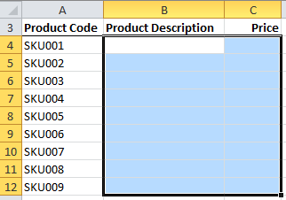
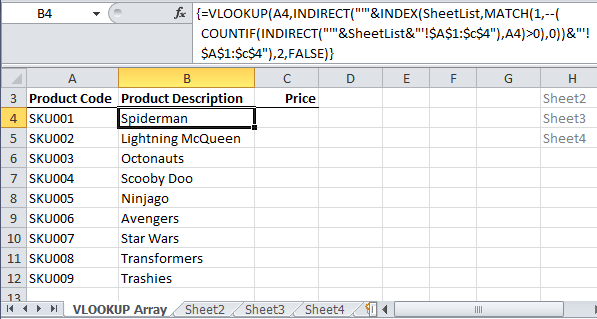
Below is our table that we want to populate by looking up the Product Code in column A and return the Product Description and Price.
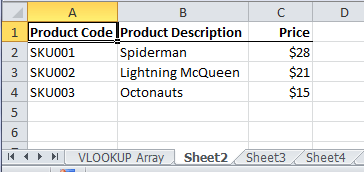
The challenge is that the product code information could be on Sheet2:
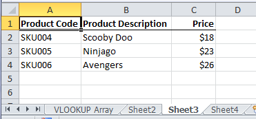
Or Sheet3:
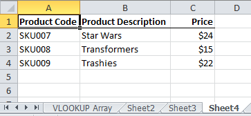
Or Sheet4:
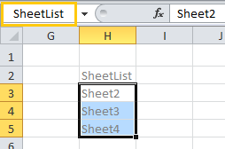
The first thing we need to do is enter a list of our sheet names somewhere in the workbook and give them a named range. I’ll give mine the very imaginative name: SheetList
Now we can enter our formula in cell B4:
=VLOOKUP(A4,INDIRECT("'"&INDEX(SheetList,MATCH(1,--(COUNTIF(INDIRECT("'"&SheetList&"'!$A$1:$c$4"),A4)>0),0))&"'!$A$1:$c$4"),2,FALSE)
It’s an array formula so we need to enter it with CTRL+SHIFT+ENTER.
We can then copy it down the column to lookup the remaining product codes.
The above is just a small sample of the toys on my boy’s Christmas lists!
How this Formula Works
Unfortunately this formula doesn't evaluate in order from left to right, so it’s a bit difficult to translate into English as I like to do, instead we’ll look at the separate components and understand what they’re doing.
First remember the syntax for the VLOOKUP Function is:
VLOOKUP(lookup_value, table_array, col_index_num, [range_lookup])
In our formula we know everything except the table_array argument. Remember we don’t know what sheet contains our lookup_value.
Instead we use the INDIRECT, INDEX, MATCH and COUNTIF functions to build the table_array reference dynamically for each product code in column A like this:
=VLOOKUP(A4,INDIRECT("'"&INDEX(SheetList,MATCH(1,--(COUNTIF(INDIRECT("'"&SheetList&"'!$A$1:$c$4"),A4)>0),0))&"'!$A$1:$c$4"),2,FALSE)
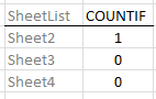
1. The COUNTIF component
The COUNTIF part of the formula is checking each sheet in the SheetList to find a match. If it finds a match it counts 1, the other sheets return a zero.
=VLOOKUP("SKU001",INDIRECT("'"&INDEX(SheetList,MATCH(1,--(COUNTIF(INDIRECT ("'"&SheetList&"'!$A$1:$c$4"),"SKU001")>0),0))&"'!$A$1:$c$4"),2,FALSE)
Our formula now looks like this:
=VLOOKUP("SKU001",INDIRECT("'"&INDEX(SheetList,MATCH(1,{1;0;0},0))&"'!$A$1:$c$4"),2,FALSE)
The {1;0;0} above represents the count of matches on the 3 rows in the SheetList. You can imagine because it found a match for SKU001 on Sheet1 it looks a bit like this:
2. MATCH Function
The syntax for the MATCH function is:
MATCH(lookup_value, lookup_array, [match_type])
From our formula: MATCH(1,{1;0;0},0)
Where zero [match_type] is an exact match.
The MATCH function is looking for the value 1 in the lookup_array {1;0;0} and returns its position. Which in this case is the first position, therefore our MATCH formula evaluates to 1 like this:
=VLOOKUP("SKU001",INDIRECT("'"&INDEX(SheetList,1)&"'!$A$1:$c$4"),2,FALSE)
Note: if it found a match on Sheet3 it would look like this:
MATCH(1,{0;1;0},0) and would evaluate to 2. i.e. the second value in the SheetList.
3. The INDEX function
INDEX Function syntax:
INDEX(reference, row_num, [column_num], [area_num])
Note: The last two arguments are optional (designated by the square brackets) and we don’t need them in this formula.
INDEX(SheetList,1)
The INDEX function uses the result from MATCH as the row number argument and returns a reference to the 1st value in the SheetList; Sheet2
Our formula now looks like this:
=VLOOKUP("SKU001",INDIRECT("'"&"Sheet2"&"'!$A$1:$c$4"),2,FALSE)
4. The INDIRECT Function
The INDIRECT Function returns a reference specified by a text string.
Everything inside the INDIRECT formula above is text, you can tell by the double quotes surrounding it. The INDIRECT function takes that text and converts it to a reference.
COUNTIF, INDEX and MATCH have done the heavy lifting, now all INDIRECT needs to do is add the necessary apostrophes to the reference and give it to VLOOKUP.
It’s a bit difficult to see the apostrophes from the double quotes so I’ve made them red below:
=VLOOKUP("SKU001",INDIRECT("'"&"Sheet2"&"'!$A$1:$c$4"),2,FALSE)
Which becomes:
=VLOOKUP("SKU001",'Sheet2'!$A$1:$c$4,2,FALSE)
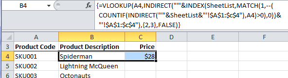
VLOOKUP Multi-cell Array Formula
Now we’ve found the product descriptions we could copy the formula into column C and change the col_index_num argument, or as Finn, my 4 year old, says ‘we could be a bit more cleverer’ and change the formula slightly so that it can find both results with the one formula!
To do this we’ll use a multi-cell array formula.
When you enter a multi-cell array formula you first select all the cells you want populated, then you enter the formula.
Since we’ve already got our formula in cell B4 we can select B4 and C4, then press F2 to edit the formula.
All we need to change is the col_index_number argument like this:
=VLOOKUP(A4,INDIRECT("'"&INDEX(SheetList,MATCH(1,--(COUNTIF(INDIRECT ("'"&SheetList&"'!$A$1:$c$4"),A4)>0),0))&"'!$A$1:$c$4"),{2,3},FALSE)
Then press CTRL+SHIFT+ENTER and you now have your price information and you have used the same formula in both B4 and C4.
Now you can copy cells B4 and C4 down columns B and C and you’re done 🙂
The Easier Option
OK, if your head is hurting here’s an easier solution that will do if you’ve only got 2 or 3 sheets to lookup.
Warning: Any more than 3 sheets and you’re susceptible to a repetitive strain injury so it’s best to use the first solution.
VLOOKUP Multiple Sheets with IFERROR
All we do is wrap the VLOOKUP formulas in an IFERROR function.
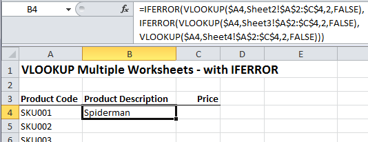
=IFERROR(VLOOKUP($A4,Sheet2!$A$2:$C$4,2,FALSE),IFERROR(VLOOKUP($A4,Sheet3!$A$2:$C$4,2,FALSE),VLOOKUP($A4,Sheet4!$A$2:$C$4,2,FALSE)))
In English it reads:
Lookup the product code in A4 on Sheet2 and return the value in column 2 of the range A2:C4, if you can’t find an exact match in Sheet2 check Sheet3, if you can’t find an exact match in Sheet3 check Sheet4.
VLOOKUP Dynamic col_index_num
The formula above is good, but we want to copy it to column C for the price and in doing so we’d need to change the col_index_num argument.
An easier way to do this is to make it dynamic by using the COLUMNS function for the col_index_num argument like this:
=IFERROR(VLOOKUP($A4,Sheet2!$A$2:$C$4,COLUMNS($A$3:B$3),FALSE),IFERROR(VLOOKUP($A4,Sheet3!$A$2:$C$4,COLUMNS($A$3:B$3),FALSE),VLOOKUP($A4,Sheet4!$A$2:$C$4,COLUMNS($A$3:B$3),FALSE)))
The COLUMNS function returns the number of columns in an array or reference.
A3:B3 = 2 columns in the range.
Therefore COLUMNS($A$3:B$3) evaluates to 2 which is the col_index_num we want.
Note how the first cell in the range $A$3 is absolute but the second cell in the range is only absolute for the row number.
Now when I copy the formula across to column C my formula dynamically updates like so:
=IFERROR(VLOOKUP($A4,Sheet2!$A$2:$C$4,COLUMNS($A$3:C$3),FALSE),IFERROR(VLOOKUP($A4,Sheet3!$A$2:$C$4,COLUMNS($A$3:C$3),FALSE),VLOOKUP($A4,Sheet4!$A$2:$C$4,COLUMNS($A$3:C$3),FALSE)))
And COLUMNS($A$3:C$3) evaluates to 3.
Enter your email address below to download the sample workbook.
If you liked this click the buttons below to share it with your friends and colleagues on Facebook, Twitter, Google+ or LinkedIn....or leave me a comment 🙂

I am trying to use the array formula and am having no luck. I can make the iferror work but not the larger the first one. I am struggling with how it finds the named range. I have tried it on a new tab, and on the sheet where the formula is being applied.
Hi Scott, we’d love to help you, but it’s difficult without seeing your file. Please post your question on our Excel forum where you can upload a file or sample file and or screenshots so we can help you further. Mynda
Dear Sir ,
I need four three sheet vlookup step please send me mail
Thank You ,
Hi,
It’s impossible to give you a meaningful answer without seeing your data.
Please start a topic on the forum and attach your workbook with the data.
regards
Phil
I have two sheets one has around 1400 names. I want to search for those names in another sheet which has 5 tabs to find out which name is available in which tab.
Hi Sakshi,
It’s impossible to give a specific answer without seeing your workbooks. Please start a topic on the forum and attach the workbooks.
Regards
Phil
I have been googling this question and cannot find any help. I know Vlookup can only find value vertically (column), and for Hlookup, horizontally (rows). What functions should I use if I want to confirm that the value in, let’s say, Column A on Sheet1 is on Sheet2, however, the values on Sheet2 are from Cells A1 through G200 (not in one column or one row).
Example: I need to confirm that the data/value of ID number “1234560” from Sheet1 is on Sheet2, regardless if “1234560” is in Cell A1 or cell C150 of Sheet2. And also, the ID number “1234560” is listed multiple times on other cells on Sheet2. I only want Excel to confirm that it is on Sheet2.
Thanks!
Hi Autumn,
You can use the SEARCH function to determine if the number exists in a range of cells that span multiple columns. The formula below assumes the number you’re checking is in cell B1 and the cells you’re looking up are on sheet2 in cells A1:D2:
=LARGE(–ISNUMBER(SEARCH(B3,Sheet2!A1:D2)),1)
If the number is found the formula will return a 1 if it’s not found it will return a zero. Note: if your lookup cell (B3) is empty and any of the cells on sheet2 in the range A2:D2 are also empty, the formula will return a 1 i.e. it will look for a blank cell and will find a blank cell.
You can change the cell references to suit your needs.
Mynda
Hi
I want to Vlookup for data in 50 sheets .
how to do that formula.
As explained above, but expanded to list all 50 sheet names.
I’m trying to apply this solution, but my sheets exist in a separate workbook. How can I modify this to work with another workbook?
Not recommended, 3d formulas will not work with closed workbooks. Best way is to bring data into your book with power query, not with formulas.
I use this formula and it works well, but what if i want to do a reverse look up? Something similar to using “Choose” where i enter information from Z1 but require the information A1 as an example?
Hi Vince,
Usually, when one needs more and more complex formulas to solve problems, it’s a strong indication that the data structure used is not optimized.
Keeping the data into the same sheet/table is the best way to store information. Of course, the data sheet must not be designed for viewing data and reports, data visualization should be separated from data storage, they hate eachother.
I suggest organizing data in a more flexible structure, it will give you much more control and more powerful reports using built in tools.
i am using this formula and it works great. I’ve set up a test excel sheet just like your example. i set the searched range to be the entire sheet, of each sheet in the sheet list, and everything works well. However, if i move your chart on sheet two, to start at B1, the formula returns #N/A. if i cut and paste the chart back to A1, the proper values are returned. is there something that isnt allowing me to recognize the lookup value if it isn’t in column a? if so, how can i allow the formula to search the entire sheet for the lookup value?
my formula:
=VLOOKUP(C5,INDIRECT(“‘”&INDEX(sheetlist,MATCH(1,–(COUNTIF(INDIRECT(“‘”&sheetlist&”‘!1:1048576″),C5)>0),0))&”‘!1:1048576”),2,FALSE)
i should clarify, i am going to be using this formula on a excel file of my own. in that file look up values could be anywhere within the sheet. So, i am hopeful there is a way to alter this formula to find the lookup value no matter where it is on the sheet.
thanks.
You will have to upload a sample file with a few manual examples, hard to visualize your data structure. Create a new topic on our forum to upload the sample file.
Hi Zach,
If the search value is in column B, then your range to search into should start from column B, VLOOKUP will always search in the first column of the range.
Hello, your Vlookup Almost works for me, the only thing i needed to add was a third value like for example:
your Formula =VLOOKUP(E2&F2,IF({1,0},First_Name&Last_Name,Grade),2,FALSE)
I want to formula= VLOOKUP(E2&F2&G2,IF({1,0},First_Name&Last_Name&Middle_Name,Grade),2,FALSE)
Is this possible? i would love to hear from you soon as its kinda urgent for work
Thanks for sharing.
Hi,
Just add a helper column with concatenated name, and use:
=Index(ColumntoReturnFrom, MATCH(E2&F2&G2,HelperColumn,0))
i want to formula for one sheet1 to another sheet 2
Can you clarify what you need?
As a Data Analyst, I found this very informative and helpful when dealing with multiple sheets and workbooks.
Keep up the great work!
Bryan
Thanks, Bryan! Glad you found it helpful.
I would like to do a Vlookup after comparing the cell value(which will have the course ID ) with that of the sheet name (course ID ) . In another worksheet will have the EMP number and course ID as cell value . It should compare the two sheet and provide me the value in the cell where course id is available . Please help as i am very new to macros
I have the below detials
Employee Number Course ID
12345 55893
23456 55893
12345 55893
23457 55893
89045 55893
Hi Farzana,
You won’t need a macro for this. However, it’s difficult to provide you with a solution without seeing your file structure. Can you please post your question on our Excel forum where you can upload a sample Excel file and we can help you further.
Mynda
I find your website too informative and useful. I became a fan of your works. Good luck for the future and thanks a lot for helping by your tutorials.
Thanks, Wahid! Glad we can help.
how can we implement vlook and drop down list linked as well as in some cases color code will be same but brands will be different(i.e paints have same color in shop but they may have many brands) or wood have the color along with that same color edge bands will be there to match) in such case how we can use vlook up table to get required sheet which we need either wood or edge band depending on color code value..
Hi Mohammed,
Please open a post o the forum and supply a workbook with data. It’s too difficult without seeing this to give you an answer.
Regards
Phil
I am trying this with google sheets. I have 5 sheets that have the same columns in them. Your formula is only looking to the first sheet of the 5 sheet list. Any idea why?
Sorry, Scott, I don’t use Google Sheets.
Hi there, it works fantastic with your example, but I closed my equivalent to Sheet1, open it again and now I can only see #N/A where my data used to be. And I cannot make it work not even by re-writing the array formula. Please advise.
Hi Marco,
INDIRECT doens’t work on closed workbooks. I recommend you consolidate your data into one sheet using Power Query.
Mynda
i have two work book and a workbook have tow worksheet means total three worksheet.
1.main sheet for vlookup
2.have two sheet as salary sheet i.pab bank ii.other bank
=vlookup(range1,table otherbank,4,0) second sheet same as other bank
how i add it in vlookup)
Hi Rohit,
You could just add two VLOOKUPs together:
=vlookup(range1,table otherbank,4,0) + vlookup(range2,table pab bank,4,0)
But ideally you would consolidate your data into a single sheet in a tabular format so you can use the SUMIF function the way it was intended.
Mynda
This article was very useful and I’ve successfully used the formula. But, are you able to pull out multiple data from multiple sheets to a single sheet. Using your example (hypothetical as I know this is SKU’s). Your formula looks for a singular match for an ‘SKU’, but what if you have the same ‘SKU’ on more than one sheet and you would like to pull out each row of data into a list? Is this possible?
Hi Paul,
It may be possible with some ugly long array formulas, but it’s not the right way to do.
You should try Power Query to bring data in the same sheet, splitting data across multiple sheets is a source of many problems.
Using complex 3d formulas is not safe, they need maintenance and they are also a potential source of errors.
Cheers,
Catalin
This article was incredibly useful! I do have one very important question, though:
What if, instead of other sheets within the same workbook, I wanted the SheetList to consist of the names of other documents? That way the formula would search a set of other excel files instead of just a set of sheets within the same workbook. How could I name those files to get the same result?
Hi Corbin,
I doubt that you can extract data from a closed workbook with these formulas.
I suggest using power query to extract data from those files, then refer your formulas to this data extract.
Catalin
hi
I have 20 files and each has 10 sheets with different names I want to get data from a files.
it is an invoice system of aluminium work.
I have drop down lists as “color” “thinness” and “model” value will be changed if one of these get changed. so the values has been already defined in other 20 files.
https://www.4shared.com/zip/Hkt7ha5iei/Invoice.html
here is sample,
the problem is I have to type vlookup formula 200 times ,
it’s awful .
but the formula works for 1 file.
please take a look in. you have definitely defined nicely but I need more clarification,I shall be very thankful to you.
please take a look in.
Hi Tayyab,
Can you upload a sample file on our forum? It will be easier to communicate and provide a useful answer. Create a new topic after sign-up to upload the sample file.
Regards,
Catalin
What if my lookup_value is in A1, and I want to return value from P22?
Hi Mark,
Hard to say without more information. Can you please post your question on our Excel Forum and include a sample Excel file so we can see your question in context and provide an answer.
Cheers,
Mynda
Hello,
I have used the above formula
=VLOOKUP(A4,INDIRECT(“‘”&INDEX(SheetList,MATCH(1,–(COUNTIF(INDIRECT(“‘”&SheetList&”‘!$A$1:$c$4″),A4)>0),0))&”‘!$A$1:$c$4”),2,FALSE)
and it worked perfectly.
But what I am trying to figure out is, what if the value that I wanted to return is not from the same row.
Like in the example I have given, lookup vallue is in A1 and I want to return value from P22.
Hi Mark,
Please upload a sample file with your data structure to our forum. It will not work with the formula you mentioned.
Currently trying to pull the data from a Work Order (WO) line from one sheet to populate into the correct fiend in another google sheet…
Trying to eliminate retype the same info into another sheet..
Can it recognize the date in the WO line and populate data into the WO line on another sheet?!?
Hi Krista,
We have no clue what that Work Order line contains. You should share a few examples, usually it is possible to write formulas to extract a specific string.
Catalin
Hello,
I have multiple file for Raw data and one main file. like below. I need to know the last name of all EMP ID from all files to main file. How can i get this in single formula, by combined the all data in one file i can get that but its time taking. can i get this without combined the data in one file?
thanks in advance.
Below is the sample for data.
file 1.
EMP ID last name first name
101 yadav naveen
102 kumar deepak
103 patel gaurav
104 sharma vivek
105 Ghosh jay
File 2.
EMP ID last name first name
101 yadav naveen
200 kumar deepak
201 patel gaurav
203 sharma vivek
main file.
EMP ID last name
101 ?
102 ?
103 ?
104 ?
105 ?
108 ?
200 ?
201 ?
202 ?
203 ?
.
Hi Naveen,
Looks like you need not only a formula that returns data from all sheets, but also removing duplicates. There is no formula to do that, maybe because it’s a bad idea to split the same type of data into multiple sheets, a poor data structure leads to very complicated formulas. I suggest keeping all the data into the same sheet, just add another column with a specific attribute (department, month, or whatever generated the need to separate them in sheets), this way your formulas will become very simple, and you will be able to use many other powerful tools,, like pivot tables, power pivots.
Catalin
Is there a way I can edit this formula to show me not just the first match found, but every match found across the sheets, and the value in the column to the right?
Hi Rebecca,
Yes, you can use this lookup and return multiple values formula, or a PivotTable…I’d use the latter every time 🙂
Mynda
HOW CAN I USE IFERROR FORMULA WITH THIS
{=VLOOKUP(A4,INDIRECT(“‘”&INDEX(SheetList,MATCH(1,–(COUNTIF(INDIRECT(“‘”&SheetList&”‘!$A$1:$c$4″),A4)>0),0))&”‘!$A$1:$c$4”),2,FALSE)}
Hi Harish,
Simply wrap your formula into IFERROR function:
=IFERROR(VLOOKUP(A4,INDIRECT(“‘”&INDEX(SheetList,MATCH(1,–(COUNTIF(INDIRECT(“‘”&SheetList&”‘!$A$1:$c$4″),A4)>0),0))&”‘!$A$1:$c$4”),2,FALSE),”Error”). Don’t forget to confirm it with CSE, it seems the be an array formula.
Hi, the formula is helpful, but what happens when in sheet 2 and sheet 3, the product description is not in column B , instead it is in Column D and G respectively?
As the files are updated regularly, the columns cannot be changed , is there a way out ? Pl guide.
Hi Rolla,
I’m afraid that the best choice for you is not a formula, you will have to use Power Query to bring the sheets data in the shape you need.
Catalin
Hi, so at my job I have to go across multiple sheets sometimes 40 + sheets, and then roll all of the data into one sheet. For example I need to know how many Finance department hours are on 40 sheets. All the sheets are structured the same with the same data in the same columns. Would I be able to use a formula from above to add up all the finance department hours and give me the total on the first sheet?
Thank you
Hi Jeffrey,
If your sheets all have the exact same structure then you don’t even need a VLOOKUP, you can just insert a SUM that picks up all of the cells between a start and end sheet. e.g. Let’s say your Summary sheet is at the beginning of the file and then you have sheets 1 to 40 that contain the department data and you want to sum the value in cell B5 on the Department sheets. The SUM formula on the summary sheet would be:
This formula would add up the values in cell B5 on sheets 1 through to 40.
Mynda
Thank you Mynda. That is actually helpful and will definitely use that in the future. I guess I should have been a little clearer. So in all of my sheets, I have different departments in column AA. So I could have a32, a33, a45, a48, a55 etc in that column, so I would be trying to find out the sun of each of those departments. So I want the total for a32, and a33 and so on.
Thank you again
Hi Jeffrey,
Ah, in that case you probably want a 3D SUMIFS: https://www.myonlinetraininghub.com/excel-3d-sumif-across-multiple-worksheets
But really what you want to do is fix the data layout so it’s not spread across multiple sheets. This is the reason you’re having to resort to complex formulas. If it were set up in a tabular format you’d be able to use a regular SUMIFS, or even better, a PivotTable. You can use Power Query to consolidate your data into a tabular format and then summarise it from there.
Mynda
This a really good formula but still not help me. 🙂
I have 4 excel sheets with employee names, employee numbers on the left column and week dates on the first row.
one work sheets will be use to gather information form other work sheets. Other work sheets have the same information but by department. on sheet 2 for example is all of the employees who work in the Production department; manager will enter a 1 in the cell related to the employee and the week when this employee will be layoff. The goal is to have all department manager update their department sheets and this information transfer to the master sheet. Could you help
Hi Leticia,
I see you’ve already posted your question to our help desk. I’ll help you further there.
Mynda
thanks for this awesome formula can you help me to lookup across workbook with sheets …
Hi there
I have used the above formula – thank you for the advice! However, can you advise on how to deal with N/A’s – that being if there are no matches on the multiple tabs the data is looking to, can the cell be left blank rather than N/A? The excel version I am using is 2010 and the data is looking over 7 tabs so therefore i am unable to use the IFERROR function.
Many thanks
Hi Ali,
Yes, you can use IFERROR to handle N/A’s.
Mynda
hi, great explanation, i took a while to land at this one, have seen the formula prior but without the explanation on the count if part.
i am having trouble adapting this approach to an index-match with 3 criteria, my formula is:
INDEX(‘sheet2!$A:$D,MATCH(sheet1!$A2&sheet1!$B2&sheet1!C$1,’sheet2′!$A:$A&’sheet2′!$B:$B&’sheet2’!$C:$C,0),4)
it works great for 1 sheet but the data is spread across multiple sheets because of the row limit in excel being “only” about 1 million
how can i use this approach with an index match instead of vlookup, i already have a list of my sheets in a named range named sheets
thanks in advance for your help
Hi Pablo,
I don’t think that Index function will work in this scenario.
The best way is to use Power Query to join all data into one table, then the formula will be much simpler than it is now. Splitting data across multiple sheets is usually a bad idea, but you don’t have many options for large data sets. A possible solution is to use IFERROR to check if data was not found in first sheet, then use in the value_iferror argument the formula to look in the next sheet. It’s not a clean solution and not dynamic, the Power Query solution looks better to me, you can try using CUBE functions to extract data from the data model.
Catalin
thank
Thanks for putting together these awesome tutorial/walkthroughs! I found this page through tons of searching and it’s the closest thing I’ve found to what I’m trying to do, but I was hoping you could help with the specific thing I’m trying to do.
Here’s a basic breakdown of what I’m trying to do:
I’ve got monthly sheets in a workbook and a specific value assigned to different names in each sheet. I want a formula that will look at each sheet and compare the values from each name and pick the largest of those values and pull all the largest values from the 3 months for each individual name into one sheet. Can this be done?
Thanks in advance!
Marc
Hi Marc,
I recommend you correct the format of your data into a Tabular layout so you can leverage the built in Excel tools to answer your questions. Your current layout does not support this.
Mynda
Hi Mynda,
I downloaded your Workbook example and experimented with it. It is exactly what I need and thanks for presenting and explaining it. How would you change this formula so it only returns one value (say just the Product description) and not the price. I want it to NOT place any result (or formula) in Col C (Price)? Anything I tried just either throws an error or places #NA in both columns. I’m new to arrays in Excel.
Hi Mike,
You have to upload your sample file with your attempts to our forum (create a new topic), to see what you did and understand what you need to do.
Catalin
Thank you, this works very well for me.. sort of..
I have my list of external workbooks (about 16 of them) and the formula works with them, finds them. BUT it will only pull from the first sheet (tab) of those external workbooks. I need it to pull from the 2nd and 3rd sheets/tabs, but nothing I do makes it work. Do you have any ideas?
Hi Dean,
Never heard about such problem. If you can return data from a sheet, you should be able to get data from any sheet from that workbook.
Can you upload a sample of your workbooks, to see what happens?
You can create a new topic on our forum.
Catalin
Hi
I wonder if you can help with this, im using the formula below to retrieve some figures, these figures will be in the same ce11 reference however the sheet 16Nov16 is the thing im having issues with. All I want is for the formula get this data from different sheets, ie 17Nov16 and 18Nov16 and so on.
=VLOOKUP(’24 Hour Summary’!$A$60,’16Nov16′!$A$1:$P$60,2,FALSE)
Thanks In advance
JoeJoe
Hi Joe,
Try this formula:
=VLOOKUP(’24 Hour Summary’!$A$60,INDIRECT(“‘”&ROW(A16)&”Nov16’!$A$1:$P$60”),2,FALSE)
You can copy it down as needed, it will recreate the day part of the sheet name.
If this is not what you wanted, you can upload a sample file on our forum.
Cheers,
Catalin
Hi,
Thank you very much for your explanation.
But I wonder if the same product code is repeated in the same sheet or different sheet, and the product price that I wanted it to come up is different, is it possible to add all the product price together?
In my case, I am trying to look up the amount of the raw material I have left in stock. But there are different lots of the same raw material. Therefore there are many duplicated cells of the same raw material that are showing the different amount in stock. I want to be able to sum up all the stocks. What should I do?
Best regards,
MM
Hi MM,
If you want to add all of the values then you’d use a 3D SUMIF.
Kind regards,
Mynda
Hi,
thank you for the nice explanation.
I was wondering why you use “- -” in front of the countif part ?
Hi Joel,
The two minus signs together are called double unary. They’re used to convert a TRUE/FALSE resulting from the >0 test into their numeric equivalents of 1 and 0 so they can be used in the MATCH part of the formula.
However, you can leave out the >0 and COUNTIF evaluates to numbers, so the double unary isn’t required. Download the file and experiment with it yourself for a better understanding.
Mynda
Hello
the formula =VLOOKUP(A4,INDIRECT(“‘”&INDEX(SheetList,MATCH(1,–(COUNTIF(INDIRECT (“‘”&SheetList&”‘!$A$1:$c$4″),A4)>0),0))&”‘!$A$1:$c$4”),{2,3},FALSE) althought complicated at first I understood it step by step. I just wanted to know if you had more variables than than just description and price, say 6 or 7 in total would the columns be {2,3,4,5,6,7,…} depending on the number of headings?
also the reference would change $A$1:$c$4 if you had more headings?
I just wanted to know would the formula change slightly with more sheets and more headings/(variables?
Thanks
Jaimal Patel
L.E.:
sry I meant, 6 or 7 sheets instead,as well as more headings?
Hi Jaimal,
You have to upgrade you data structure to a more flexible format, seems like your file has the CFN syndrom (Complex Formulas Needed), this happens usually when source data is split into multiple sheets, for visual and printing purposes. If you decide to upgrade your structure, you will be able to use the most powerful excel tool for data processing and reporting.
You can try the new support forum, if you upload a sample file with your data structure, we will certainly find new solutions for you.
Here is the link to our forum: myonlinetraininghub.com/excel-forum
Catalin
Thankyou Catalin
Jaimal Patel
Dear Madam,
refer to your sheet is it possible to get the first occurrence of an id (by time at what time he entered first) or use some formulas/functions to do so.
Hi Prem,
Can you please upload a sample file on our forum? Here is the link to the Excel forum
Catalin
yes ma’am I can upload the same.
know there is another question in mind related to your vlookup with multiple sheets.
Is it possible to use match function at col_index_num as I am using formula but it now works. =IFERROR(VLOOKUP($K2,INDIRECT(“‘”&INDEX(range,MATCH(1,–(COUNTIF(INDIRECT(“‘”&range&”‘!I:I”),$K2)>0),0))&”‘!I:O”),MATCH(1,–(COUNTIF(INDIRECT(“‘”&range&”‘!I:O”),$K2)>0),0),0),””) is there any way to do it such as we can do this in simple vlookup
Hi Prem,
The need for complex formulas is a known disease, generated by a poor data structure. To get your data well, and improve its health, you have to change it to a more flexible data structure. If the structure is correct, there is no need for complex formulas. Not to mention that you will be able to use more powerful built in tools to analyze the data. If you have same data structure in all those sheets, then the best choice is to reformat them with Power Query. Only then you will see the real power of modern excel.
You can upload a sample file on our new forum, we can help you find a solution there: myonlinetraininghub.com/excel-forum
Catalin
How can I adjust this approach for the following?:
I have the same lookup criteria that I want to find on every other sheet in my workbook. How can I adjust this formula to display the maximum result found amongst all the sheets? The term being looked up could appear in any row on the later sheets (I haven’t built the sheet yet or I’d give specific references). Can it be done with just INDEX – MATCH formulas instead of VLOOKUP?
Hi Mark,
Can you please upload a sample file on our Help Desk? (create a new ticket). It will be easier for us to understand how the data is structured and provide a personalized answer to help you.
Catalin
This is all very helpful.
However, what do we do if the length of data (the number of rows) in each sheet is different than the other. Sheet 1 has 300 rows, sheet 2 has 140 rows, sheet 3 has 1000.
Will the formula change
=VLOOKUP(A4,INDIRECT(“‘”&INDEX(SheetList,MATCH(1,–(COUNTIF(INDIRECT(“‘”&SheetList&”‘!$A$1:$c$1000″),A4)>0),0))&”‘!$A$1:$c$1000”),2,FALSE)
I am assuming that I will go with the largest number of rows. but then that would mean that i will have empty rows in the other sheets.
Please help!
Hi Rmango,
Correct. Just adjust your formula range to fit the largest number of rows. It doesn’t matter if some sheets have blank rows in that range.
Mynda
I AM HAVING AN ERROR IN DUPLICATNG THE FORMULA. ALTHOUGH THESE ARE DIFFERENT WORKBOOKS, THEY WILL BE OPEN WHEN PERFORMING THE LOOKUP.
I AM GETTING THE MESSAGE THAT THERE ARE TOO MANY OR TOO FEW ARGUMENTS.
COULD YOU PLEASE ASSIST? BELOW IS THE FORMULA I AM USING.
=IFERROR(VLOOKUP($A2,'[ASCEND template FY Q1 2016.xlsx]6. Payout by worked hrs’!$A$1:$Y$4314,11,FALSE),IFERROR(VLOOKUP($A2,'[ASCEND template FY Q2 2016.xlsx]6. Payout by worked hrs’!$A$1:$Y$4314,11,FALSE),IFERROR(VLOOKUP($A2,'[ASCEND template FY Q3 2016.xlsx]6. Payout by worked hrs-Q3-16 ‘!$A$1:$Y$4314,11,FALSE), IFERROR(VLOOKUP($A2,'[ASCEND template FY Q4 2016.xlsx]6. Payout by worked hrs’!$A$1:$Y$4314,11,FALSE),IFERROR(VLOOKUP($A2,'[ASCEND template FY Q1 2017.xlsx]6. Payout by worked hrs’!$A$1:$Y$4314,11,FALSE))))
Hi,
Your formula should have a value for the last IFERROR, the formula should end like this:
IFERROR(VLOOKUP($A2,'[ASCEND template FY Q1 2017.xlsx]6. Payout by worked hrs’!$A$1:$Y$4314,11,FALSE),””))))
You can upload a sample file on our Help Desk, (create a new ticket), if you need more help on this problem.
Catalin
Not sure if you are still monitoring this thread. I came across your solution while working on a summary sheet that has to pull and display a value for the “current month” from one of 12 additional sheets in the workbook. Each of the 12 additional sheets contains data for one month of the year. The “current month” value in my summary sheet changes each month automatically based on the “system-month.”
I tried using your formula to get Excel to go find the sheet with the name matching the “current month” and then look up a value in the appropriate monthly sheet. The value I am looking up is located in the same cell in every sheet.
Unfortunately, it doesn’t work. In debugging it gets partly through, identifying the month I am looking for, looking at my SheetList, but then I get a #VALUE! error. Here’s a copy of your formula follow by my formula reflecting my values.
VLOOKUP(A4,INDIRECT(“‘”&INDEX(SheetList,MATCH(1,–(COUNTIF(INDIRECT(“‘”&SheetList&”‘!$A$1:$c$4″),A4)>0),0))&”‘!$A$1:$c$4”),2,FALSE)
VLOOKUP($AA$41,INDIRECT(“‘”&INDEX(SheetList,MATCH(1,–(COUNTIF(INDIRECT(“‘”&SheetList&”‘!$AC$4:$AN$4″),A4)>0),0))&”‘!$AC$4:$AN$4”),4,TRUE)
I thought the problem was the A4 in the last third of the formula. Assuming it was supposed to be the same value as the value in the first A4 in your formula, I changed mine to $AA$41. I still get the same error.
I tried simplifying and doing a straight vlookup with the name of the specific sheet embedded in the lookup and that works. But I need the INDIRECT function to find the correct month so I don’t have to update my formula everything month.
L.E.: One additional thing… I did hit Ctrl, Shift, Enter and then I get an #NA… regardless of which cell reference I use.
Can you help?
Thank you.
Jim
Hi Jim,
Can you please upload the file on our Help Desk System? You can create a new ticket, it will be easier to find an answer to your problem.
Cheers,
Catalin
Do the spreadsheets you are searching have to be in the same workbook?
How would you set the array to look up spreadsheets in different folders?
Thanks,
Maurice
Hi Maurice,
INDIRECT won’t work on worksheets in closed external workbooks. For this reason I don’t recommend this method. It would be much safer to consolidate your data first.
Kind regards,
Mynda
Thank you for your reply. I think you’re right – I should consolidate all of my different .xlsx files into one workbook with several tabs across the bottom.
Then Incan run your INDIRECT script on all of this data.
How do I consolidate many files in different folders into one workbook?
Thanks,
Maurice.
Hi Maurice,
Actually, I’d even consolidate the separate worksheet tabs into one. You’ve got over 1M rows so unless you’ve got masses of data then it should be in one worksheet.
This is how all of Excel’s tools were designed to work: PivotTables, functions etc. It’s when you start splitting data out that you run into problems, as you’ve found. Using INDIRECT, while it works, is really not the right way to summarise your data, it’s like putting a band-aid on.
I write about the ideal data format here: https://www.myonlinetraininghub.com/excel-tabular-data-format
You can use Power Query to consolidate data, or you can get an add-in to consolidate your worksheets and workbooks, or you can do it the manual way and copy and paste.
I hope that helps point you in the right direction. Let me know if you have any questions.
Mynda
Dear Sir,
I am trying to solve below query but message is display #NA. Please guide me now on my mail.
=VLOOKUP(AND($G$6,$H$6),’Vacant Only’!$A$4:$N$221,14,FALSE)
Hi Binoy,
You can’t use AND like that. I presume what you want may be:
But without seeing your data it’s a guess. This tutorial might have the answer:
https://www.myonlinetraininghub.com/vlookup-multiple-values-in-multiple-columns
or this one:
https://www.myonlinetraininghub.com/vlookup-multiple-values
If none of those help then you can send a sample file via the Help Desk.
Kind regards,
Mynda
Sheet1
G6 H6
Inst_Code course_code
4 16
4 16
4 16
Sheet2
A5 C5 N5
Inst_Code course_code Vacant
4 16 1
4 16 1
4 16 1
I use =VLOOKUP($G$6&$H$6,’Vacant Only’!$A$4:$N$221,14,FALSE) then Answer is display #NA. Please guide me.
Hi Binoy,
You need this formula:
Entered as an array formula with CTRL+SHIFT+ENTER
Explained here under the heading ‘VLOOKUP vs INDEX & MATCH’:
https://www.myonlinetraininghub.com/vlookup-multiple-values-in-multiple-columns
An Excel file submitted via the help desk would be easier to answer as I could refer to cell references.
Kind regards,
Mynda
Sheet1
Inst_Code course_code
4 16
4 16
4 16
4 16
4 17
4 17
4 22
4 22
4 23
4 28
4 28
4 29
Sheet2
Inst_Code Course_Code Vacant
4 16 1
4 16 1
4 17 3
4 17 2
4 23 2
4 29 1
=INDEX(‘Vacant Only’!$A$4:$N$221,(MATCH(‘Vacant Only’!$G$6&$H$6,’Closer of OPEN CAt Final’!$G$6&$H$6,0)))
As per your guide lite I use this formula in my Excel sheet but Error message showing #NA.
Please guide me. Please reply as early as possible in my mail as well in post.
Binoy,
The first argument of INDEX should only be one column, the column containing the data you want to return i.e. ‘Vacant’. Then also make sure you enter the formula by pressing CTRL+SHIFT+ENTER.
This is an array formula. It should have curly braces surrounding it after entering, which are only visible in the formula bar.
If you continue to have problems please do not reply here. Post your question with supporting Excel file via the Help Desk.
Mynda
Still I am waiting for your reply. Please give answer urgently.
I have replied, but I can’t give you a specific answer without a specific example in a workbook.
Mynda
First of all this formula is awesome. Along with your 3D SUMIF, this is amazing. Someone asked in Excelforum.com if there was a way to expand this to include multiple criteria. I figured that out by changing your COUNTIF to a COUNTIFS. I just wanted to post this here in case anyone else has the same question of how to lookup multiple criteria.
I put the single quotes and the exclaimation point in the text of the list to make the formula a little easier to read.
=VLOOKUP(A2,INDIRECT(INDEX(Sheets&"$A$1:$C$1000",MATCH(1,COUNTIFS(INDIRECT(Sheets&"$A$1:$A$1000"),A2,INDIRECT(Sheets&"$B$1:$B$1000"),B2),0))),3,0)Thanks, Nigel. Appreciate you sharing your formula too.
Cheers,
Mynda
I’ve been searching and searching for a solution, and here it is! FINALLY!!! You are AMAZING!!!!
🙂 Thanks! Glad I could help.
Hi Mynda,
I am not sure what happened to my post from earlier today but thank you for responding. My original post asked about using the formula above in a way to look across 35 sheets 1st for the date in cell A3 and then when it finds the right date it then pulls the sales, traffic, conversion etc.
You mentioned that it would be very hard to do this and I should try putting everything in tabular data format. However, the only problem with that is that there is a lot of other information on each sheet that is needed and cannot be put into tabular form (not all numbers). Could I lead with the find function to find the date?
Again, thanks for your help.
Hi Jim,
A Tabular data set can have numeric and text data. It really is the ‘only’ way you should store data for use in formulas in Excel. Any other way and you just run into problems as you are now.
But to answer your question, looking up a date is no different to looking up any other value/text. You just reference the cell containing the date you want to lookup and then reference the range of cells containing the dates. If it’s not working then I suspect there is an inconsistency with your date formats. I can’t tell without the workbook but you can send it to me via the Help Desk.
BTW, your comment in at the bottom of the blog post where you originally entered it.
Kind regards,
Mynda
Thank you again for taking the time to reply, I really appreciate it.
I am going to try that and a few more ideas and see where it takes me. If I still run into the problem then maybe send it to you via the help desk.
Yes, sorry about the double comment. For some reason when I was looking at the page my original response was not at the bottom top or middle. Even did Control F and searched by name and nothing. Then after submitting the new post it popped up and was there. Lastly, thank you for all the videos and webinars on dashboards…they have really helped me at work!
You’re welcome, Jim.
Hi,
This might be what i have been looking for, however still a little confused.
I have 35 (1 for each day and 1 weekly conversion tool) worksheets that consist of sales data and some other daily information. I want to create a monthly worksheet that will auto populate each night once the sales have been entered.
On my monthly overview sheet, I have day of the week and date listed. Is there a way that i can use this formula to first search all 35 sheets for the date and when it finds the correct date it then pulls the sales info?
Thanks for any help!
Hi Jim,
You could use this formula but the best thing you can do is put all your data onto one sheet. You are making Excel work extra hard (and yourself) by formatting your data across 35 sheets.
I recommend you read this tutorial on Tabular Data. Tabular data is the secret to an easy Excel life 🙂
Mynda
Oh my head is going to explode and my eyes have glazed over. How in the world do you keep your sanity?
😀 Sorry about that, George. Sometimes banging your head on the desk gives some light relief!
Brilliant formula!
Can this be used when I have all the data in one workbook and the values I am matching against are in another?
I tried to incorporate the path name in front of the named range but this just created an error with two few arguments.
Thanks
Hi Daniel,
Unfortunately, you can’t use names to reference ranges in closed workbooks.
Catalin
You can use IFERROR with Index Match formulas — something like this
IFERROR(INDEX(‘Sheet2’!$B$2:$B$4,MATCH($A$4,’Sheet2 ‘!$A$2:$A$4,FALSE),0),IFERROR(INDEX(‘Sheet3’!$B$2:$B$4,MATCH($A$4,’Sheet3!$A$2:$A$4,FALSE),0),IFERROR(INDEX(‘Sheet4′!$B$2:$B$4,MATCH($A$4,’Sheet4’!$A$2:$A$6,FALSE),0),0)))
Hi Michael,
That’s an INDEX & MATCH version of the ‘VLOOKUP Multiple Sheets with IFERROR’ option above.
Thanks for sharing.
Mynda
Thank you for your kind words
Another way of doing it is with If(ISERROR Here’s the VLookup version with IF(ISERROR
=IF(ISERROR(VLOOKUP($A$4,’SHEET2′!$A$2:$C$4,2,FALSE)),IF(ISERROR(VLOOKUP($A$4,’SHEET3′!$A$2:$C$4,2,FALSE)),IF(ISERROR(VLOOKUP($A$4,’SHEET4′!$A$2:$C$4,2,FALSE)),0,(VLOOKUP($A$4,’SHEET4′!$A$2:$C$4,2,FALSE))),(VLOOKUP($A$4,’SHEET3′!$A$2:$C$4,2,FALSE))),(VLOOKUP($A$4,’SHEET2′!$A$2:$C$4,2,FALSE)))
The IFERROR version goes from left to right, while the IF(ISERROR version goes from the center out.
Hi,
Is there a cut-off point with the number of sheets that method one becomes not optimal to use (i.e. 10 sheets with 100k rows each)? At that point would it be better to use a macro or some other method?
Hi Steven,
I haven’t tested the formula on large volumes of data so it’s hard to say. One thing I would consider is consolidating your data into one sheet, as it should be.
This formula is necessary because the data isn’t stored in a single tabular format. It’s spread over multiple sheets which is a no-no.
Kind regards,
Mynda
Unfortunately,the data that I am trying to match up against is larger than the Excel row limit therefore I needed to break out to multiple sheets.
Ah, sounds like time for a database then. How about putting your data in Access and using PivotTables to summarise it?
Mynda
Hello, I see this is an old article, but I was hoping you could help me…
I have a formula that searches 1 worksheet in the document and displays all rows that which meet a certain criteria for 1 of 3 columns.
=IFERROR(INDEX(HHBN!B$2:B$622,SMALL(IF(HHBN!$E$2:$E$622=$C$1,ROW(HHBN!B$2:B$622)-ROW(HHBN!B$2)+1,IF(HHBN!$M$2:$M$622=$C$1,ROW(HHBN!B$2:B$622)-ROW(HHBN!B$2)+1,IF(HHBN!$AC$2:$AC$622=$C$1,ROW(HHBN!B$2:B$622)-ROW(HHBN!B$2)+1))),ROWS(HHBN!B$2:HHBN!B2))),””)
I’m trying to incorporate your idea here of searching through all four tabs, but I can’t get it to work. Thank you for any help you can give.
Hi Robert,
Please upload a sample workbook with your data structure and details on what are you trying to achieve. It’s almost impossible to see why your formula is not working. You can use our Help Desk.
Catalin
Catalin,
Thank you for the response. The formula I posted works how it is suppose to. I was hoping to use the idea in this post to adjust it so it will search all tabs instead of just one, but I can’t figure it out. I’ll try to upload it to the help desk. Thank you again for your response.
Robert
Ok Robert, i’ll wait for that file and details, we’ll find a solution for you.
Cheers,
Catalin
since i was high school and colleges, I only now we learn this vlookup but it’s difficult when you getting started until the next steps so we need more time to learn and study this vlookup.
Hi Randy,
It’s all about practice. The more you do it the easier it will get.
Cheers,
Mynda.
Hi Mynda –
This is similar to a challenge I am experiencing – with a little twist.
I am trying to lookup data in a Workbook based on the value of two cells in a Worksheet.
Here is the example:
Worksheet ‘A’, cell C8 contains the letter “P”.
Workbook ‘B’ contains 26 worksheets – A thru Z.
1. Go to the worksheet in Workbook ‘B’ based on the letter in cell C8.
2. Lookup the value of cell D8 in the same worksheet.
3. Array:Workbook ‘B’, Worksheets A-Z,$C:$H,6,0
I would appreciate any assistance you can offer.
Thanx!
Hi Joe,
Please upload a sample workbook on Help Desk
This way we can work on a real data structure, and the result is not just an idea.
Thank you for understanding.
Catalin
Try this
=INDIRECT(“‘[WorkbookB.xlsx]”&C8&”‘!$d$8:$D$8”)
sheet1 in total then sheet 2 in total then i give a sheet1+sheet2 total in sheet3 plz ans me with example plz
Hi Jinal,
For example, if the total value for sheet1 is in cell E14, and same for sheet2, you can use a 3D SUM to add the totals from sheets 1 and 2:
=SUM(Sheet1:Sheet2!E14)
If it’s not what you wanted, please use our Help Desk to upload a sample workbook with detailed description of what you are trying to achieve.
Catalin
Superb! Wow!
Thanks, Robert 🙂
Very useful step by step explanation, even the beginners can do well
Thanks, Ajeshkumar 🙂 Glad you liked it.
Mynda.
Hi Mynda,
This is very usefull. But along the same lines I would like to use similar formula to access the data from different excel reports (stored in various folders) instead of sheets in a same workbook.
For examples, my files are saved here:
c:\2013\Nov13\a.xls
c:\2013\Nov13\b.xls
c:\2013\Nov13\c.xls
c:\2013\Nov13\d.xls
Formula:
=VLOOKUP(BI20,INDIRECT(“‘”&INDEX(SheetList3,MATCH(1,–(COUNTIF(INDIRECT(“‘”&SheetList3&”‘!$A$1:$c$9″),BI20)>0),0))&”‘!$A$1:$c$9”),2,FALSE)
SheetList3:
c:\2013\Nov13\a.xls
c:\2013\Nov13\b.xls
c:\2013\Nov13\c.xls
c:\2013\Nov13\d.xls
I tried using the above entries in a SheetList but the formula didn’t work. How should I do this ? Do I need to put the file name in double/single quotes, etc. ? I’ve tried everything but it didn’t work.
Thanks
Hasan
Hi Hassan,
Please provide a sample of your workbooks, so i can test on your environement, this way you will have a faster solution.
You can use the Help Desk: https://www.myonlinetraininghub.com/helpdesk/
Cheers, Catalin
Hi, i have a workbook with 6 sheets, each sheet has 15 colums & approx 6000 rows of data, so i want to run a vlookup for a specific criteria but the consition is that the formula should check all the 6 sheets before giving the result, is that possible??
Hi Rajanz,
Yes, it’s possible using the formula in the blog post above. Note: it will only work if the match is only one one sheet in your workbook. If you have multiple matches it won’t return the correct result.
Kind regards,
Mynda.
Hi Mynda,
I tried applying the formula to my worksheet but it doesnt return any value, i unable to debug the error, would it possible to look at the sheet & suggest a solution?
Hi Rajanz,
You can send me the workbook via the help desk and I’ll take a look. Please include specific instructions on what you’re trying to do and give me an example of your expected result.
Thanks,
Mynda.
I am using this formula to look over many pages and for some reason it works on some of the cells but others it either returns a value of “#N/a” or “0”. What is the difference between the two?
Hi Chase,
A #N/A error means the lookup_value cannot be found. A zero means it found the lookup_value but the cell you asked it o returned was either empty or contained a zero.
I hope that helps.
Kind regards,
Mynda.
I read the previous post.. and success! sorry to bother. Thanks 🙂
Cheers, Kevin. Glad you figured it out.
Hey, I understand about 70% of this and am still re-reading it to fully understand. Is there a way however to use this formula.. but refer to a seperate workbook for the alternating sheets?
Topic: Excel Lookup, Multiple Sheets
All we need to change is the col_index_number argument like this:
=VLOOKUP(A4,INDIRECT(“‘”&INDEX(SheetList,MATCH(1,–(COUNTIF(INDIRECT (“‘”&SheetList&”‘!$A$1:$c$4″),A4)>0),0))&”‘!$A$1:$c$4”),{2,3},FALSE)
How does the above formula evaluate {2,3}?? I have always typed the column number I needed.
Thanks in advance.
P.S. Your website is fantastic!!
Hi Brad,
Thanks for your kind words. Glad you like our site 🙂
The formula you’re referring to is a multi-cell array formula. i.e. the formula is entered in multiple cells all at once.
Because we’re entering the same formula in both columns (Product description & price), we need to give it the col_index_number for both columns. This is the {2,3} information in the formula (known as an array constant). The array formula knows to use 2 for the Product Description column and 3 for the Price column.
I hope that helps.
Kind regards,
Mynda.
Mynda,
Thanks for this formula! I was able to get it to work when everything is in the same workbook, but the application I’m using it for has so many sheets that I want to separate them into two workbooks. I can’t get the reference to work. Basically, this is what I have:
=VLOOKUP($B3,INDIRECT(“‘”&INDEX(‘[workbook2.xlsx]Sheet1’!SheetList,(MATCH(1,–(COUNTIF(INDIRECT(“‘”&'[workbook2.xlsx]SheetList’!SheetList&”‘!$c$8:$d$8″),$B3)>0),0)))&”‘!$c$8:d$8”),2,FALSE)
Any suggestions?
Hi Steve,
Does your SheetList contain the workbook name as well as the sheet name?
INDIRECT is deriving the range to be looked up but since it’s in another workbook it also needs the worksheet name, not just the sheet name.
Kind regards,
Mynda.
Thanks for the reply. I thought of that, so I tried with an unnamed list as well, and just dragged a copy of the sheet over to a new workbook so it would update the address automatically. So the list started out as:
Students!$B$3:$B$34
…and became:
‘[Equipment Checkout.xlsx]Students’!$B$3:$B$34
Here, “Students” is the worksheet with the list of sheet names on it (from B3:B34), each sheet is named after a student, and “Equipment Checkout” is the workbook that contains the sheets. When I drag one of the equipment inventories (Sleeping Bags, for example) over to a new book, it changes the list address as above, but I still get #n/a. Just can’t figure this one out.
Thanks for your help.
I thought about your response and tried something new, still to no avail. I put the workbook name “Equipment” in cell B2 and changed the list to B2:B34. I still get the #n/a error.
Is that what you meant?
Hi Steve,
I got this formula to work:
=VLOOKUP(A7,INDIRECT(“‘”&INDEX(Book3!sheetlist,MATCH(1,–(COUNTIF(INDIRECT(“‘”&Book3!sheetlist&”‘!$A$1:$c$4″),A7)>0),0))&”‘!$A$1:$c$4”),3,FALSE)
Where my ‘sheetlist’ is in Book3.xlsx. How does that compare to what you’ve tried?
Mynda.
I tried that and still had trouble, but I did find a solution after thinking about your last post! Like you did, I put the workbook in the formula, and all I had to do was put the workbook location in front of every item on the sheetlist. So instead of just sheet1, sheet2, etc. the list looks like Drive:Folder:[workbook.xlsx]sheet1.
Now it works perfectly. Thanks for your help!
Brilliant! Glad you got there in the end 🙂
Hi Mynda,
Slight variation… how do I check where a value is present in multiple sheets?
Your IFERROR/VLOOKUP solution stops at soon as it find a hit. I want to keep going and make sure I find another hit.
I’ve tried COUNTIFS, VLOOKUPS, SUMPRODUCT and MATCH… but they don’t work as the value I’m looking for is not always in the same position in both tables, ie. the code could be the 2nd row in the first sheet/array and in the 18th row in the second sheet/array.
Please help… can’t find the answer.
Thanks,
Steven.
Hi Steven,
Do you want to sum these multiple instances of a match? If so the 3D SUMIFS might be what you’re after.
If that’s not it please send me a sample file via the help desk so I can see what you’re working with.
Cheers,
Mynda.
Mynda,
This is super helpful but how would I edit this if the sheets I’m trying to access are in another workbook? I understand indirect doesn’t work unless the other workbook is open (unless I download the add-on that lets you do so). Any help would be greatly appreciated!
Woops never mind, just read the comment above!
🙂 Cheers, Chris.
Hi this is great and really helpful but currently i have a vlookup to search another workbook which has ever increasing amounts of rows.
The number of rows have reach their maximum so now it is recording data on a second sheet.
My question is can you use this to look up multiple sheets on another workbook?
thanks in advance
jim
Hi Jim,
If you’re running out of rows it sounds like it’s time to put all that data into Access.
I imagine you can use that formula across multiple workbooks but you’d have to add the workbook name in front of the worksheet name so that the INDIRECT function had the correct cell address.
The reference would look a bit like this:
Where the workbook name is inside [square brackets].
Also, the formula will only work when both workbooks are open. INDIRECT doesn’t work if referencing a closed workbook.
I hope that helps. Let me know if you get stuck and I’ll take a look.
Kind regards,
Mynda.
Really helpful, lucid, attractive and cool…
Thank you, Shyam 🙂
Thanks, Shyam 🙂
Thank you. It worked quite well; however, my spreadsheet has 50 worksheets & the formula works only for the the 1st ten, although the the named range I created contains all the 50 worksheets. Is there any way to make it check all the 50 worksheets?
Appreciate your help.
Hi Rodolfo,
Not sure why it wouldn’t work for all 50 sheets. Are you able to send me the file via the help desk or is it too big?
Cheers,
Mynda.
That is brilliant.
Could you pls further explain what’s the purpose of –(,>0)?
As I find that the formula seems working properly without it; but interestingly if I change input the formula as array with Column Index {2,3}, it doesn’t work…
So what is the magic of the –??
Appreciate your explanation! 🙂
Hi MF,
Well spotted. If you don’t use the >0 test you can also omit the double unary –, so the formula would become:
=VLOOKUP(A4,INDIRECT("'"&INDEX(SheetList,MATCH(1,(COUNTIF(INDIRECT("'"&SheetList&"'!$A$1:$c$4"),A4)),0))&"'!$A$1:$c$4"),2,FALSE)The double unary converts TRUE/FALSE outcomes (resulting from the >0 test) to 1’s and 0’s so they can be used in the MATCH part of the formula. By leaving out the >0 the COUNTIF evaluates to numbers, so the double unary isn’t required.
I hope that helps.
Kind regards,
Mynda.
THANKS A LOT
IT IS VERY GOOD EXAMPLE AND MUCH USEFUL DON’T KNOW ANY THING PEOPLE ALSO.
thanks
Param
Cheers, Param 🙂
Dear Sir/Madam,
I would like to learn “Vlookup” formula.. i have preparing many statment, it is take more time to do and completed, if i know how to use the vlookup formula into it, it will help us to time saving. The problem is No. 1. For Example: while the employees resigned the job next month when we will going to prepare the employees register i need the current employees name list excepted the resigned employees.
Please help me. Thank you!
Best Regards,
S.SIMBU.,
Chennai-Tamil Nadu-INDIA
Hi Silambara San.s,
You’ll need to send your file to the help desk so we can see exactly how it is laid out. Please also provide clear instructions to help us understand your needs.
Kind regards,
Mynda.
This was GREAT!!!! Been trying to figure out how to write a nested formula for thisl
Cheers, Duane 🙂
Very, very cool and perfect for a logistics solution that I am putting together.
However, I am not able to recreate the Excel array solution on a google spreadsheet. Do you have any idea why that would be? I get a a parse error.
Thank you
Hi Kent,
As much as we would want to shed some light on your problem,
We don’t have much expertise to our disposal regarding Google spreadsheets.
All I know is that not all of Excel’s functions will work with Google;hence,
It really depends on what funtions you’re using.
Cheers,
CarloE
Now that Google has significantly changed their Sheets app, can you shed light now on how this can be done? I tried to do this in Google Sheets and the only stumbling block (after hitting ctrl-shift-enter) was that the MATCH parameter was not recognized: “Did not find value ‘1’ in MATCH evaluation.”
Thanks!
John
Hi John,
Sorry, I’m not familiar with Google Sheets. Only Excel 🙂
Kind regards,
Mynda
Hey John,
I’m having the same problem as yours. Been looking for a solution the last couple of the days with little success so far. Have ultimately found a solution to this problem?
Regards
Nothing yet Christophe
But I am monitoring it because it’s solving a number of problems with clients that only work with Google Docs. This is perhaps in the wrong forum…
If I find out more, I will come back…
nice sharng
Hi Owais,
Nice words. Thank you, on behalf of Mynda.
Cheers.
CarloE
Hi Mynda,
Great code… works like a charm..
But I have one issue.. I am using VBA and the number is sheets which will have the data is not known in the beginning… so my query is
1. How do i create a named array at run time
2. how do i insert the formula in the cell using VBA
3. This formula gives rsults only if I insert it in the cell and press ctrl+shift+ enter in each cell individually… if i drag then i dnt get the results.
Awaiting your comments on the same
Hi Mohit,
1. To create a named array:
Horizontal
    ActiveWorkbook.Names.Add Name:="RunTime", RefersToR1C1:= _
        "={""jay"",""wash""}"
or Vertical
    ActiveWorkbook.Names.Add Name:="RunTime", RefersToR1C1:= _
        "={""jay"";""wash""}"
2. Code to put contants to array to a range (I presume you already know how to add a commandbutton because you said you’re using VBA). I’m saying this anyway: Add a commandbutton and copy&paste the code as applicable(Horizontal, Vertical)
how to add commandbutton
Horizontal
   Dim s As Variant
   s = Evaluate(ThisWorkbook.Names("RunTime").RefersTo)
   Range("A1:B1").value = s
or Vertical
   Dim s As Variant
   s = Evaluate(ThisWorkbook.Names("RunTime").RefersTo)
   Range("A1:A2").value = s
3. Regarding this… are you having problem with this one? lol.
I am not in the proper position to answer you this because I am
not one of the creators of Excel. To give you a hint however, named arrays
are not technically arrays but constants;hence, if you notice I used the Evaluate()
function to put it into an array. Think about the transpose function… you’ll get
the idea. And please, there’s nothing we can do about it.
Cheers.
Carlo
Dear Carlo,
Many thanks for your inputs.
I got my doubts clarified by googling a bit.
Regarding point 2, guess my question was not clear.
What I want to know is,
If I insert it manually in a cell I will type
=VLOOKUP(A4,INDIRECT(“‘”&INDEX(SheetList,MATCH(1,–(COUNTIF(INDIRECT(“‘”&SheetList&”‘!$A$1:$c$4″),A4)>0),0))&”‘!$A$1:$c$4”),2,FALSE)
and press ctrl+shift+enter
But if I want to insert this through VBA I will have to insert the command
Range(“A1”).FormulaArray = “eqivalent of the VLOOKUP formula” and then loop this statement till the end of the sheet.
now what I want to know is what will be the eqivalent of this VLOOKUP formula???
Hi Mohit,
LOLz.I could hardly see that was your intended question. I thought you were relating 2 from 1.
Anyways…. so much of semantics….
Try this:
Range("A1").FormulaArray = _
        "=VLOOKUP(R[-13]C[-3],INDIRECT(""'""&INDEX(SheetList,MATCH(1,–(COUNTIF(INDIRECT(""'""&SheetList&""'!$A$1:$C$4""),R[-13]C[-3])>0),0))&""'!$A$1:$c$4""),2,FALSE)"

Range("A1").AutoFill Destination:=Range("D17:D21"), Type:=xlFillDefault
Note: This is the equivalent of your formula in this post :=VLOOKUP(A4,INDIRECT(“‘”&INDEX(SheetList,MATCH(1,–(COUNTIF(INDIRECT(“‘”&SheetList&”‘!$A$1:$c$4″),A4)>0),0))&”‘!$A$1:$c$4″),2,FALSE)
Cheers.
CarloE
PS: I really didn’t get to troubleshoot the formula because I don’t have the data that will perform the INDIRECT & Match function to return
the table array… hence it is returning an Error.But if you’ll put this all in a commandbutton, this will show the formula that you presented to me
in this post. If this will function in yours, then good. If not, you might as well send your file through HELP DESK. so we can give you the exact formula you need!!!
I am trying to do vlookup and hlookup together. I need to get the exact figure for a column and row from another sheet, please help I am stuck. Thank you
Hi Francie,
Please try this formula:
                Kobe the black mamba's stats last 5 games
  B       C       D      E        F      G
2		Points Per Quarter
3		 1	2	3	4
4Team Vs Utah	 15	5	10	0
5	 Phoenix 16	6	11	1
6	 Chicago 17	7	12	2
7	 OKC     18	8	13	3
8	 Miami	 19	9	14	4


Team Vs:Chicago	(C11)
Quarter: 3	(C12)

Score(Formula):=VLOOKUP(C11,C4:G8,MATCH(C12,D3:G3)+1,FALSE) result:12
The data is B2:G8 including the headers Points Per Quarter and Team Vs
The lookup values are in C11 and C12. You may just hardcode the lookupvalues like this
=VLOOKUP("Chicago",C4:G8,MATCH(3,D3:G3)+1,FALSE)Read More VLOOKUP’s
Cheers.
CarloE
Awesome Mynda, thank you very much.
You’re most welcome, Debbie 🙂
HI Mynda
As always, how to make the hard and complicated formula’s look easy, with a step by step break down, I’ve been using excel since 1996, and still I find new tricks and tips (inspired by you blog)
Thank you
Regards
Adam
🙂 Wow, thanks Adam.
Hi Mynda, I can’t seem to make the formula work.
Can I send you my excel file so you may kindly check where I went wrong?
Please….
Thanks 🙂
Hi Lhey,
Sure, please send your file via the help desk.
Kind regards,
Mynda.
Hi Mynda,
It’s working now. Just made a mistake in the Name Range part.
Your formula is awesome!
Thanks,
Lhey
Great 🙂 Glad you got it working.
Hello Mynda, I have gone through the various tricks and techniques. The VLOOKUP for multiple sheets is an excellent piece and the way you have explained is terrific!!! I am advanced excel user but after going through your tricks, I really feel that you are Goddess of Excel in front of whom I am dwarf. Thanks dear for your tips on excel.
You’re welcome. Thanks for your kind words, Mehul 🙂
Question- How could this formula be revised to allow for this scenario.
For example what if “Spiderman” was on multiple tabs. Only one tab would have a cost associated. For example sheet2 value 0, sheet3 value $28.00.
The formula; as is would return 0, ie returns the first match, but what I want is to return the $28 from sheet3
Hi Philip,
You can use the 3D SUMIF formula for this.
Kind regards,
Mynda.
Thank you for your succinct solution
You’re welcome, Philip 🙂
If you’d like to take this one step further, on my site here where that same technique is demonstrated there is an additional application that uses that same technique to create a dynamic HYPERLINK in an adjacent cell that you can click to jump directly to the data on that specific sheet.
Thanks for sharing, Jerry 🙂
just looking at this gives me a headache 🙁
🙂 this is quite an advanced formula, Tristan. Maybe start off with a regular VLOOKUP first.
The data was very useful, but the formula looks too lengthy.
Hi Renjini,
Thanks for your feedback. Have you got an alternative? Perhaps you’d like to share it.
Cheers,
Mynda.
Countif is a function amazing … and here great use with indirect function … I had never seen it work so. Thanks Mynda, good trick!
Thanks, r. Glad you liked it 🙂
Fantastic
Cheers, Tahir 🙂