Each time I write a tutorial I use the Google Keyword tool to find search phrases that are relevant. I use these phrases as tags on my post to help you find it easier in Google and other search engines.
The Google keyword tool spits out a list of phrases which I then export into Excel like the example below.
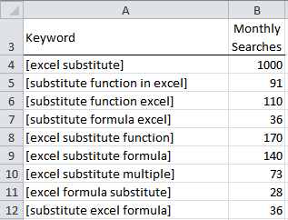
Then from the list above I need to create a list of comma separated phrases.
The problem is I first need to remove the square brackets and then I need to join all of the phrases together separated by a comma and a space.
There are a few ways I can do this.
- Use Text to Columns to remove the square brackets then use a CONCATENATE or & (ampersand) formula to join the text together, or
- Use Find & Replace and then CONCATENATE to join the text together, or another way is to
- Use the SUBSTITUTE function to remove the square brackets and then join the text together using a cheeky Find and Replace trick in Microsoft Word.
Since most people know how to use Find & Replace (if you don’t, sign up for our online training here), and I’ve already written a tutorial on CONCATENATE, I’m going to cover the SUBSTITUTE function today.
How to Use SUBSTITUTE
First let’s tackle the text in cell A4 which is [excel substitute]
In cell C4 I will enter the following SUBSTITUTE Formula:
=SUBSTITUTE(SUBSTITUTE(A4,"[","",1),"]",", ",1)
Result:
excel substitute,
This formula is actually using the SUBSTITUTE function to replace multiple items.
The SUBSTITUTE formula in orange is replacing the left square bracket with nothing and the SUBSTITUTE formula in blue is replacing the right square bracket with a comma and a space.
How the SUBSTITUTE Function Works
SUBSTITUTE Function Syntax
=SUBSTITUTE(text, old_text, new_text, [instance_num])
Where:
Text = the cell the text is in
Old_text = the text you want to replace. You need to put this in “double quotes”. Note this is case sensitive.
New_text = the new text you want. Again, in double quotes. If you want to replace it with nothing then simply enter two double quotes “”.
Instance_num = this specifies which occurrence of old_text you want to replace. If omitted, every instance of old_text is replaced.
Ok, now I have my formula in cell C4 I can copy it down the column then I’m ready to join the text together.
How to Join the Text Together
This is almost blasphemy for a devout Excel fan, but this is the quickest way so here goes!
- Copy your new text from column C.
- Open Microsoft Word…take a deep breath as you go to the other side
- In Word Paste special > Unformatted Text
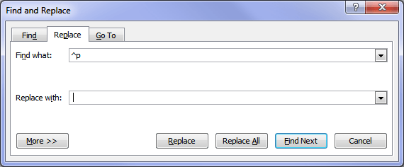
- CTRL+H (for Find & Replace)
- Enter a ^p in the ‘Find what’ box. ^p is the end of the paragraph in Word.
- Enter nothing in the ‘Replace with’ box.
Tada… your text now looks like this:
excel substitute, substitute function in excel, substitute function excel, substitute formula excel, excel substitute function, excel substitute formula, excel substitute multiple, excel formula substitute, substitute excel formula,
You might be saying to yourself that I could have done that all in Word using Find & Replace and you’d be right, but that would be admitting that Word is better at some things than Excel and I can’t bring myself to do that 🙂 Plus you wouldn’t have learnt how to use the SUBSTITUTE function.


To replace line breaks within a single cell within Excel use Find & Replace with ^j instead of ^p as you would in MS Word.
Nice tip, Doug. Thanks for sharing.
Mynda
Well, true, Mynda, but wouldn’t it just be easier to paste the original Keyword text straight into Word and use F&R to remove the square brackets also?
regards,
Excel fan
Help please!
Using Microsoft 2013, is there a quick and easy way to remove ALL non-printing characters in one easy action? The CLEAN formula was only designed to remove the first 32 non-printing characters in the 7-bit ASCII code (values 0 through 31) from text and in the Unicode character set, there are additional non-printing characters (values 127, 129, 141, 143, 144, and 157).
The main character that causes me issues is the HTML entity; (character 160). I used to use Find to search for spaces I can’t see using Alt while keying in 0160 – then I’d manually remove any spaces if I could find them. I presume the SUBSTITUTE formula is similar, without the manual part.
My issue is that every type of character needs to ‘substituted’ individually. Is there a way to do them all at once?
Hoping someone can help
Thank you
Hi Aimee,
You can try a simple macro, that will replace all chars in a single run, in all worksheets:
Sub FindReplace()Dim Wks As Worksheet
Dim FindWhat As Variant
Dim Chars As Variant, i As Integer
Chars = Array(127, 129, 141, 143, 144, 157, 160)
For Each Wks In ActiveWorkbook.Worksheets
For i = 0 To 31 ' replace chars from 0 to 31
Wks.Cells.Replace what:=Chr(i), Replacement:="", _
LookAt:=xlPart, SearchOrder:=xlByRows, MatchCase:=False, _
SearchFormat:=False, ReplaceFormat:=False
Next i
For i = 0 To UBound(Chars) ' replace the chars listed in array
Wks.Cells.Replace what:=Chars(i), Replacement:="", _
LookAt:=xlPart, SearchOrder:=xlByRows, MatchCase:=False, _
SearchFormat:=False, ReplaceFormat:=False
Next i
Next WksThere are 2 loops, one to remove the chars from 0 to 31, and another to replace the chars from the Chars array: Chars = Array(127, 129, 141, 143, 144, 157, 160)
You can add any char codes to this list.
Cheers,
Catalin
SUBSTITUTE(SUBSTITUTE(A4,”[“,””,1),”]”,”, “,1) You have indicated what the orange and blue formula is doing in this; however, I am confused with why you indicated the instance number of 1 because there is only 1 instance of each of the brackets; one bracket is [ and one bracket is ]. I removed the 1 and I got a reference error.
Thanks
Hi Wanda,
You can remove the 1 from both instances of SUBSTITUTE function, but don’t forget to remove the argument separator for that argument (the comma). Remove “,1” instead of just “1”.
Cheers,
Catalin
Hello,
This SUBSTITUTE function may be able to help me, but it seems limited somewhat. Is there something easier that can help me look at a range of cells, compare the data and then replace it accordingly?
For example, look at all cells A1:A10 and if they contain ABC replace it with ‘1’, if they contain DEF replace it with ‘2’ and if they contain GHI replace it with ‘3’ etc etc. Anything other than values specified should display “N/A” or “NULL”.
I don’t want to use IF because there are 82 values to compare and replace, and the initial range they are located in, may be anywhere between 10 cells or 100 cells.
Essentially, I am looking at creating a macro where I highlight the cells, run the macro and the change happens.
Thank you for your assistance.
Hi John,
That sounds like something I can do with a macro. If you can send me your workbook so I can see the data it would make it easier for me to write the code.
If you create a Helpdesk ticket you can attach the workbook to that https://www.myonlinetraininghub.com/help-desk
Regards
Phil