There’s no built-in way to create Excel Slicers for fiscal years, however the solution is easily achieved by adding an extra column to your source data to classify each date into its relevant fiscal year.
Download the Workbook
Enter your email address below to download the sample workbook.
Watch the Video
Be sure to watch to the end for the bloopers!
Creating Excel Slicers for Fiscal Years
In Australia our financial year runs from July 1 to June 30 so I’ll use that as my example.
In columns A and B below is the data I want to analyse in a PivotTable and Pivot Chart; it’s the trading volume of some stocks by date.
And in columns E and F is my lookup table (with the named range tbl_fiscal_yr), that I’ll use to map the dates in column A into their Fiscal Period:
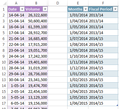
Note: Both tables are formatted as an Excel Table and my dates are dd-mm-yy.
I'll add a column (C) to classify the dates in column A into their fiscal year. For this we can use a VLOOKUP formula with a Sorted List:
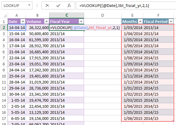
Note: If the formula arguments like [@Date] look odd to you it’s because they’re using the Excel Table’s Structured References.
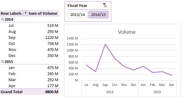
Now that we have the new column (C) for the fiscal year we can use that field for the Slicer and then choose the fiscal year we want to display in the PivotTable and Pivot Chart:

Hi Mynda,
Our fiscal year starts in November. I found a solution by having a “month” column with the first day of the corresponding month, then setting the column to a custom format “mmm” in the table. That format carries forwards to the slicer, keeping the months in the order I want 🙂 Unfortunately, this doesn’t work for power pivot, so I’m trying to find a way to do there too.
Hi Daniel,
In Power Pivot you add a numeric column to your table with the sort order e.g. November will be 1. Then set the ‘Sort By’ for the Month column name to be sorted by the numeric column.
Mynda
Hi Mynda. The difficulty I’m having when I do a pivot table is that the months still show in a calendar year order despite my classifying them in the way you suggested. Could it be because the figures I’m using are monthly figures only – ie there is only one date for each month. Anyway I’m trying to get the figures into an April/March fiscal year but I get them sorted January/December with the last 3 months of the fiscal year showing as the 1st 3 months of the calendar year.
Maybe I’m missing something.
Hi Peter,
Having just one entry for each month won’t be the problem. In your PivotTable do you have the calendar year and calendar month in the rows area and the Fiscal year in the Slicer or Filter area like my example at the bottom of the post?
If you’re still stuck please post your question and file on our Excel forum where we can help you further.
Mynda
Thank you for your help Mynda. That worked!
I should have looked a bit more closely.
Regards
Peter
No worries, glad that fixed it.
Thanks for this Mynda.
I work at a sugar refinery and our working day starts at 8AM therefore anything produced from midnight to 8AM gets booked to the previous day’s production.
Also our production week starts at 8AM on Monday morning.
I can adapt this idea to accommodate this.
Thanks for sharing your hard work and experience. Your video’s and examples are great.
glad I could help 🙂
Very interesting
Hi Mynda, The videos are very helpful and easier to follow than reading through the text. the headshots are good at the beginning and end of the video, but distracting during the training portion. As always, your training material is very useable. Please keep including the videos!
Thanks for all your hard work on the training material!
Bob T
Thanks, Bob. Glad you’re finding the videos helpful.
Mynda
Mynda
This is just fantastic.
Your Newsletters are marvelous.
Keep it up.
Thanks, Dennis! Glad you like it 🙂
Mynda
Hi Mynda,
Following the videos is way easier than reading the blog, so please keep the videos. Also it does help to see your facial expressions as you explain things, it makes it more real.
I love that you added a blooper at the end, great sense of humor.
Thanks for sharing so much knowledge, and for your hard work, your material and explanations are the best.
Keep up the good work.
Pablo
Thank you, Pablo! I’m glad you found the video easy to follow and liked the personal touch 🙂
Very good and appreciated! Thanks!
Cheers, Mike.
I do find the headshot a little distracting but it is nice to see your face at the beginning and at the end of the video. The bloopers are a nice touch.
Including the head shot is fine, in my opinion. Creates a good connection with your students.
BR
great tutorial again Mynda thank you.
Yes your head-shot is a bit distracting after a little while, maybe just have it run for a minute or so by way of introduction, i would add that the background fades in and out colour wise which is not flattering to you, if i may be so bold.
And as my dear old Pop used to say
awrabest
Hi Mynda
Ascertaining and using a fiscal year value (as opposed to a calendar year) for a given date is a frequent task for us bean counters, and for me even more so now as a financial analyst when building models with time-series data for valuations, DCFs, etc.
However, rather than build a separate table and lookup that table for the Fiscal Year as you have demonstrated, I usually just add a formula where the value is required to directly return the calendar year of the end of fiscal year date (e.g. return 2015 for any date between 01/07/14 and 30/06/15). A single number is much easier to work with mathematically than the two year format like 2014/15.
So in your tbl_stocks, I’d use the following formula in column C instead of the VLOOKUP:
=YEAR([Date])+IF(MONTH([Date])>=7,1,0)
Re the headshot in the video: I don’t believe it adds any value whilst the focus of attention needs to be on the content, but does make for a greater connection at the end during the wind up. It is a little distracting to me during the guts of the presentation, and means you have to be very careful with your facial expressions and other things you might do unconsciously whilst talking!!) You could consider doing a fade-out after the intro and then zoom back in for the wind up.
Cheers
Col
Hi Col,
Thanks for sharing your formula. There are many ways to skin the Excel cat, so to speak.
I think I will try the fade in/out for the headshot in the video as you and others have suggested. It sure will take the pressure off while recording, too 🙂
Cheers,
Mynda
Hi. I think the vlookup array for the fiscal year exercise could be trimmed to two rows:
Months Fiscal Period
1/3/2014 2013/14
1/1/2015 2014/15
Since a looked-up date that falls between two lookup array values in the first column reverts to the smaller value, I think the above array would suffice.
Thanks,
Abbott Katz
Hi Abbott,
Good point. I could certainly trim it to:
1/3/2014 2013/14
1/7/2014 2014/15
Since our fiscal year runs Jul 1 through Jun 30.
Cheers,
Mynda
I vote to keep your face on the videos … not at all distracting and it tends to create a more “classroom/Personal touch” feeling. The videos are simply terrific, btw.
Thanks for the video feedback, Dan, Dennis, Bruce and Alex.
I think next time I’ll try the fade in/out so I’m not there the whole time. I did find I got in the way of the PivotTable field list so finding somewhere to place the camera shot was tricky.
Cheers,
Mynda