Last week Keith asked how he can ignore blanks in a range referenced by a Data Validation list.
I think you’ll agree the list below on the right with the blanks removed looks a lot nicer.
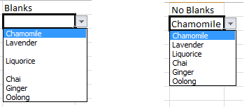
Extract a List Excluding Blank Cells
To get the ‘no blanks’ look we first need to create a new list that excludes the blanks.
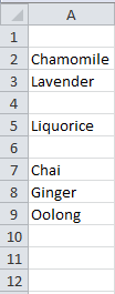
Here’s our original list containing blanks starting in cell A2 through to A9:
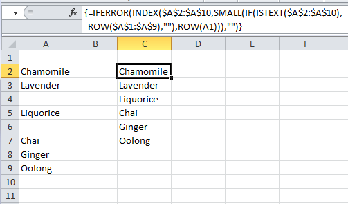
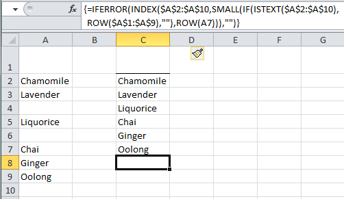
And in column C we’ll create our new list that excludes the blanks.
Stop looking at the formula bar, I don’t want to put you off 🙂
Formula to Extract a List Excluding Blanks
The formula in cell C2 is:
=IFERROR(INDEX($A$2:$A$10,SMALL(IF(ISTEXT($A$2:$A$10),ROW($A$1:$A$9),""),ROW(A1))),"")
And in English it reads:
Look at the range A2:A10 and return the first value if it is text (i.e. not blank and not a number). If this formula returns an error just enter nothing (as denoted by the "").
This is an array formula so it needs to be entered by pressing CTRL+SHIFT+ENTER, then copy down to remaining rows.
SMALL’s Big Role
Let’s expand on the SMALL(IF(ISTEXT part of the formula first:
=IFERROR(INDEX($A$2:$A$10,SMALL(IF({TRUE;TRUE;FALSE;TRUE;FALSE;TRUE;TRUE;TRUE;FALSE},{1;2;3;4;5;6;7;8;9},""),{1})),"")
The SMALL function syntax is:
=SMALL(array,k)
We’ve used the IF function to return the array argument. More on that in a moment.
The k argument is the position in the array we want to find. i.e. 1 is the smallest, 2 the next smallest and so on.
You’ll notice in our formula we used ROW(A1) to dynamically return the k argument. i.e. ROW(A1) simply evaluates to 1 and returns the first value in the list that isn’t blank.
We use ROW(A1) so that as we copy the formula down column C the ROW function reference will go up in increments of 1 (because the reference to A1 is relative, not absolute).
So, in cell C3 the ROW function part of the formula will be ROW(A2) which evaluates to 2 and will return the second value in the list that isn’t blank, and so on.
IF Function
The IF part of the formula first identifies which cells in the range contain text by using the ISTEXT function to test the cells in the range A2:A10.
If the cell does contain text it returns a TRUE, and if not it returns a FALSE, which you can see in orange below:
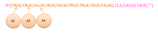
In the list above the first TRUE is referring to cell A2, the next TRUE refers to A3, and the first FALSE refers to A4 and so on.
Whilst this ISTEXT function is evaluated inside the formula, it might be easier to visualise how it works if we insert the formula in column B like this:
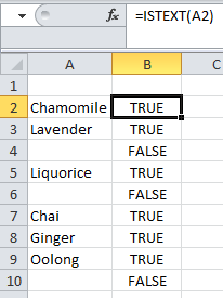
That list of TRUE’s and FALSE’s in column B is the same as the list in the IF formula.
Now, because we actually need a list of cell numbers that contain text (for the SMALL function’s ‘array’ argument), as opposed to TRUE/FALSE values returned by the ISTEXT function, we use ROW($A$1:$A$9) to return an array of numbers 1 through 9 like this:
{1;2;3;4;5;6;7;8;9}
Note: we need 9 numbers because there are 9 cells in the range A2:A10.
Next the IF function finishes evaluating and returns an array of numbers that represent the cell numbers in the range A2:A10 that contain text like this:
=IFERROR(INDEX($A$2:$A$10,SMALL({1;2;"";4;"";6;7;8;""},ROW(A1))),"")
Again, we can see how Excel does this if we put the different components of the formula in separate columns in our workbook:
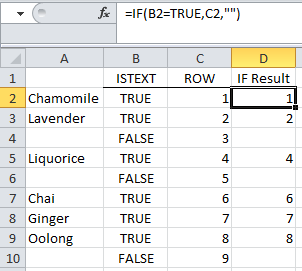
That is; rows 1,2,4,6,7 and 8 in the range A2:A10 contain text.
Next the SMALL function finishes evaluating and goes from this:
=IFERROR(INDEX($A$2:$A$10,SMALL({1;2;"";4;"";6;7;8;""},{1})),"")
To this:
=IFERROR(INDEX($A$2:$A$10, 1),"")
INDEX’s Turn
Now finally INDEX knows which value to return from the range A2:A10, which is the first value.
Remember the syntax for INDEX is:
INDEX(reference, row_num, [column_num], [area_num])
=IFERROR(INDEX($A$2:$A$10, 1),"")
Note: We’re only using the first two arguments for INDEX. The column_num and area_num are optional arguments as denoted by the square brackets.
IFERROR - The Fall Guy
IFERROR picks up the pieces if there is an error in the result and simply returns a blank.
This is important because the next thing you need to do is copy this formula down column C to at least row 10 (because later on you might enter values in cells A4, A6 and A10).
However, because there are currently only 6 values in column A you would end up with errors in cells C8:C10 if you don’t use IFERROR.
Download the Workbook
Enter your email address below to download the sample workbook.
Inside the workbook is an option that ignores blanks instead of the example above which relies on finding text.
This is useful if your data isn’t text, or is a combination of text and numbers.
Next week we’ll look at how we can use this list in a Data Validation list that ignores the blank cells at the end. i.e. cells C8:C10 in our example above.


Hi Mynda,
Thank you for your tutorials.
For this topic, Excel validation lists that excludes blanks from range, do you have a workaround using Excel 365’s new functions.
Would Unique & Filter work in the Data Validation source box?
Hi Uma,
Yes, this is a very old post! You’re right, you can use FILTER to omit blanks in a data validation list.
Mynda
I have tried this formula over and over with only the first result being accurate. Once I drag down the formula to additional cells, I get a #NUM error within the SMALL portion of the formula. When evaluating the formula, the range will read true with double quotes and a zero with a false result. Can you please help me find the error in what I am doing? Please contact me via email and I can send you what I am working on to see how it is searching. Thanks!
Hi James,
You can create a new topic on our forum after sign-up and upload your sample file so we can see what’s wrong.
See you there!
Cheers,
Catalin
I’m trying to use this technique. My data in column A of your example is equal to cells on another worksheet within the same workbook. The blank cells from the source get copied as a Zero (0) in the A column in your example. I then use an IF formula to remove the zeros using the null string “”. When I apply this technique it does not work because the cells with the null string are not actually blank. I’ve confirmed this by using ISBLANK to see if that was the issue.
Can you recommend a way to create a new column that removes the cells with the null strings?
Thanks.
Hi Tom,
Please see this tutorial on ignoring blanks returned by formulas. If you get stuck please post your question on our Excel forum where you can also upload a sample file and we can help you further.
Mynda
Mynda,
Thanks for your reply.
After I posted my question, I read through several of the comments on this post. I came across a reply saying to replace the ISTEXT with LEN()>0 in the formula to remove blanks. This was successful.
I’ve learned that Excel treats blank cells differently. If a cell has a formula that produces a null “” result, the cell appears to be ‘blank.’ However, if you apply ISTEXT, or ISBLANK to that cell a TRUE and FALSE result is respectfully returned. But, LEN() applied to the cell returns 0.
If I understand Excel’s behavior, the ISTEXT and ISBLANK formula apply to the contents of the cell that may be displayed in the formula bar, but not necessarily what is displayed in the cell after calculations. However, the LEN formula only applies to contents displayed in the cell after calculations.
Since the formula in this tutorial to remove blank cells was dependent on a 0 value to work, ie a FALSE for ISTEXT, the same result was obtained by using LEN() for a cell with the null “”.
Thanks for the reply and for a straight forward explanation of how this formula works.
Tom
I have seen in below comments how to make the cells auto populate when referencing data on a separate tab, I have used the below formula with no success.
=IFERROR(INDEX(‘5. Information Gathering’!$E$10:$E$16,SMALL(IF(ISTEXT(‘5. Information Gathering’!$E$10:$E$16),ROW(‘5. Information Gathering’!$E$10:$E$16),””),ROW(‘5. Information Gathering’!E10))),””)
No data is returned at all
The data range on the ‘Information gathering’ tab I have starts at cell E10 which I see starts causing an error. When i use the same above formula without any data in the top row in that tab and the tab I am trying to formulate the data it works without issue.
Is there any issue with the data trying to read it from a few rows down?
Hi Jayden,
You’ve misunderstood the purpose of the ROW function. Under the heading ‘SMALL’s Big Role’ I explain what ROW is doing. Please read this again. Hopefully you’ll see that it should be:
=IFERROR(INDEX('5. Information Gathering'!$E$10:$E$16,SMALL(IF(ISTEXT('5. Information Gathering'!$E$10:$E$16),ROW('5. Information Gathering'!$A$1:$A$7),""),ROW('5. Information Gathering'!A1))),"")Mynda
Would this formula work on multiple colums?
No, sorry, Jay.
Thank you
You’re welcome
I tried this in a spreadsheet in Excel 2007, inside a table, It only worked on the first line. I modified it to fit the cells I used. The cells that have Text also has a formula in it that pulls text from another cell. The spreadsheet is used to create song lists from a list of 200 songs. I used a check mark control to select the song for the list. this moves the Text to another column. The problem is the column will have blank spaces. Your Formula is what I need but I do not know what condition is breaking the formula.
Hi Dave, please post your question and Excel file on our forum where we can help you further.
Mynda
Help please! I’m trying to write a formula that will skip blanks in column A and Concatenate cells G thru M of the row containing information in Column A. Thanks
Hi J,
Please post your question and a sample Excel file containing an extract of your data and desired result on our Excel Forum where we can help you further.
Thanks,
Mynda
So similarly I am using the formula posted in another response for cells that have formulas in them. But for whatever reason I am only getting an output of #NAME? The column of data is in A2:A9 with a header in A1, and the formulas for removing the blanks from A2:A9 are in C2:C9 with a header in C1 as well. My formulas in A2:A9 are simple =If statements looking for data in B2:B9 (will be replaced in different sheet once I learn how this stuff works! lol)
The formula is
=IFERROR(INDEX($A$2:$A$9, SMALL(IF(LEN($A$2:$A$9)=0,””, ROW($A$2:$A$9)-MIN(ROW($A$2:$A$9))+1), ROW(A1))),””)
But if I change the =0 to =1 then it will copy the column over, but will not exclude the spaces.
=IFERROR(INDEX($A$2:$A$9,SMALL(IF(LEN($A$2:$A$9)=1,””,ROW($A$2:$A$9)-MIN(ROW($A$2:$A$9))+1),ROW(A1))),””)
Not sure what I need to do to get this to work.
Hi Kyle,
Upload a sample file with your data and formulas so we can see what’s wrong. Use our forum, just create a new topic after sign-up.
WHAT SHOULD BE THE FORMULA WHEN THE CELLS CONTAINS FORMULA WHICH ARE BLANKS??
Hi,
Instead of IF(IsText($A$2:$A$9), use IF(LEN($A$2:$A$9)>0
There are more versions, see comments below.
=IFERROR(INDEX($J$7:$J$34,SMALL(IF(ISTEXT($J$7:$J$34),COLUMN($J$7:$J$34),””),ROW(A1))),””)
always error in formula and blocked the ” $J$34,SMALL ” why?
Hi Victor,
Excel might be using the semicolon “;” as arguments separator in functions, not the comma “,”. Replace all commas with semicolon.
I have data in C10:O10 with blanks between them. I want to consolidate and copy this information vertically into cells B2:B5. Whats the formula to get the data consolidated in a column?
Hi Darin,
The formula is very similar:
=IFERROR(INDEX($C$10:$O$10,SMALL(IF(ISTEXT($C$10:$O$10),COLUMN($A$10:$M$10),””),ROW(A1))),””)
Hi Catalin, Thank you for the quick reply. I’m getting blanks with the formula and I saved it as an array formula. I have dates in various cells in a single row that I want to reference in another sheet but consolidated. Is the A10:M10, correct?
Hi Darin, do a test in same sheet, then move the references to the other sheet after you’re sure it works as expected.
A10:M10 is correct, it’s just to get an index number starting from 1, to be used in SMALL function. Column (A10) will return 1, and this will return the first value. If this range does not start with the first column(row in previous version) , first values will be missing from the output.
Does not matter where A10:M10 is coming from. It can be in current sheet, or in any sheet like Sheet1!A10:M10, the result will always be a number from 1 to 12.
If you have in C10:O10 formulas that returns zero length strings like “”, please keep in mind that those are NOT blanks.
See the comments below for versions that can deal with those formula results.
Catalin
Hi Catalin, So, I think I know the problem… does IsText consider numbers or dates? because I tested with replacing the dates with names and they showed up using the formula. my data looks like c10 has 9/5/19 and a few cells over 9/6/19, etc… I’m thinking maybe Isblank would work better? I don’t have any formulas in-between the dates… Thanks again for all your help!
If you look at the comments below, you will see the version that fits for you, as mentioned previously.
Instead of IF(ISTEXT($C$10:$O$10),COLUMN($A$10:$M$10),””) , use:
IF(LEN($C$10:$O$10)=0,””,COLUMN($A$10:$M$10) . this version will work for zero length strings as well as for blanks/empty cells.
I’m getting this result: using the IsNontext formula is bringing in the date but it’s also picking up blanks as the 1/0/00.
9/5/19
1/0/00
1/0/00
9/6/19
1/0/00
I want to see:
9/5/19
9/6/19
9/7/19
etc…
Good to understand this, but the issue I have is that my ‘blank’ cells aren’t truly blank. They contain formulas from an IFERROR function throughout the range. Excel therefore treats these as populated cells, so my still contains lots of blanks. Is there a way around this?
Hi Hils,
When there is a formula that returns zero length strings “”, those are not seen as blanks, but you can evaluate instead the length of the text in that cell:
=IFERROR(INDEX($A$2:$A$9, SMALL(IF(LEN($A$2:$A$9)=0,””, ROW($A$2:$A$9)-MIN(ROW($A$2:$A$9))+1), ROW(A1))),””)
Hi Guys. Thanks for this. I finally got it to work with a new fresh list but when i use a list that is first using a formula to generate it just puts the listed item in the correlating cell. So my list in Column A is a list made up from another worksheet and made using the following formula – =IF(D151=”n”,B151,””) – This is one line of around 50 to generate a list that has a ‘N’ in column ‘D’. I then copy this list again using a standard ‘=’ formula to another sheet into column A and using the above formula in column ‘C’ cut as described here it just copies the listed item across on the same row. Do i take it this formula of yours will not work if it is using a formulated list?
I do hope that all makes sense and thanks in advance for your help.
Hi John,
See the comments below, the question was asked before:
When there is a formula that returns zero length strings “”, those are not seen as blanks, but you can evaluate instead the length of the text in that cell:
=IFERROR(INDEX($A$2:$A$9, SMALL(IF(LEN($A$2:$A$9)=0,””, ROW($A$2:$A$9)-MIN(ROW($A$2:$A$9))+1), ROW(A1))),””)
Hello
I have tried your formula and it works great but…. how did you define “listIndex” and “listOffset”?
I saw in your sample excel file that in “data validation” you chose “list” and as “source” you typed in “listIndex” or “listOffset”
When I do it, excel tells me that : named range u specified cannow be found.
Can you help?
Thanks
Hi Tom,
listIndex and listOffset are named ranges.
Mynda
I have an error “too few arguments”
That means one of the functions is missing an argument. You’ll have to check the formula carefully to make sure it’s the same as mine.
Hi,
I’m trying to use this formula but keep running into issues the result is either a “0” or nothing. One issue is the table I’m trying to copy has a formula in it. The idea is to copy one list to another tab removing all the blanks or where the formula doesn’t have a response. So, the table is J5 to J136 and here is the formula in J5 “=VLOOKUP(B5,G1:H111,2,FALSE)” that formula continues down to J136. Below are my two attempts:
=IFERROR(INDEX(Recipes!J5:J136,SMALL(IF(ISTEXT(Recipes!J5:J136),ROW(Recipes!J5:J136),””),ROW(Recipes!J1))),””)
=IFERROR(INDEX(Recipes!$J$5:$J$136,SMALL(IF(LEN(Recipes!$J$5:$J$136)=0,””,ROW(Recipes!$J$5:$J$136)-MIN(ROW(Recipes!$J$5:$J$136))+1),ROW(Recipes!J1))),””)
Thank you for any help and if I need to I can post to the forum if necessary.
Cheers,
Westley
Hi Westley,
Please post your question and supporting Excel file on our forum where we can help you further.
Thanks,
Mynda
I am just getting the first number repeated
Hi Matt,
It’s tricky to diagnose without knowing more. Can you please post your question on our Excel Forum where you can share your Excel file.
Thanks,
Mynda
Hi,
Really Struggling to get this to work in any other part of the spreadsheet except your original ranges, when I copied the test works perfectly , when I try to apply it to my spreadsheet – nothing, can you help please, I have uplodaed the file
Hi Richard,
Where did you upload your file to? If you posted it on our Excel forum then someone will look at it there.
Mynda
Hi
I have downloaded the template and extended the ranges but this seems only to be able to handle three spaces before it gives up
Is there anything I should be doing?
Hi Karen,
We have to see what you have, can you upload your sample file on our forum?
I downloaded the template, but the formulas weren’t working. When I clicked into a formula cell and hit enter, your result disappeared. Is there an option in excel that needs to be turned on to get your formula to work? I haven’t had any luck in translating your results.
Hi Matt,
The formula dissapeared because it’s an array formula, not a regular formula. As it says in the article:
“This is an array formula so it needs to be entered by pressing CTRL+SHIFT+ENTER, then copy down to remaining rows.”
A simple Enter will break the array formula, turning it into a normal formula.
tried using this but doesn’t work when cell has formula. is there a way to make it work with formula in cell that displays blank.
i think i have the formula if condition and “” if not true
Hi Delos,
When there is a formula that returns zero length strings, those are not seen as blanks, but you can evaluate instead the length of the text in that cell:
=IFERROR(INDEX($A$2:$A$9, SMALL(IF(LEN($A$2:$A$9)=0,””, ROW($A$2:$A$9)-MIN(ROW($A$2:$A$9))+1), ROW(A1))),””)
Dear Concern want to share my problem i have the screen shot but i cant paste here (system not supporting). How ill sent that screen shot?
waiting for your reply.
Regards
Hi Syed,
Please post your question on our Excel forum where you can share screenshots and files.
Thanks,
Mynda
Hello,
Can you give me a function returning the row number for which the cell content is not blank in a specific column?
Thanks a lot!
MVDB
Hi,
The formula to remove blanks from a range is this one:
=IFERROR(INDEX($A$2:$A$9, SMALL(IF(LEN($A$2:$A$9)=0,””, ROW($A$2:$A$9)-MIN(ROW($A$2:$A$9))+1), ROW(A1))),””)
You can easily modify it to do the opposite, returning only the row numbers of the blnk cells:
=IFERROR(INDEX(ROW($A$2:$A$9), SMALL(IF(LEN($A$2:$A$9)<>0,””, ROW($A$2:$A$9)-MIN(ROW($A$2:$A$9))+1), ROW(A1))),””)
As you can see, there is a very small change.
Cheers,
Catalin
I replicated this example exactly by copying and pasting the formula and creating an exact copy of the table…..and I cannot get any cell to output after “Chamomile”.
Hi Joseph,
This is an array formula. Did you enter the formula by pressing CTRL, SHIFT and ENTER keys at the same time?
Mynda
This is the new feature which only available in excel 10. You can easily remove blank cells from a range as it allows you to delete the row. these formulas help me lot while i am working in spreadsheets.
Hi Nick,
Glad you found the formulas helpful, although this isn’t a new feature only available in Excel 2010. IFERROR was available in Excel 2007 too.
Mynda
One thing is not clear in your instructions. You must array enter ONLY the first cell of your new list, then copy the formulas down. It took me an hour and another search to learn that. It would be good to place such a comment right before you first show the formula. Some like me never quite read the whole article unless what we first try doesn’t succeed. Thank you for helping.
Hi Clifton,
Sorry for the confusion. I’ve expanded on the instructions after CTRL+SHIFT+ENTER…
If you’re ever stuck like that then feel free to ask us so you don’t waste time.
Mynda
I used a variation of this formula to search a column for blank cells and if true then to output the cell value from another column. The issue I’m seeing is if there are 2 blank cells in a row the 2nd value isn’t returning the value but instead 0.00 – any idea why that might occur? My data set is in another tab.
Formula
=IFERROR(INDEX(Quality_Investigations!M$2:M$1000,SMALL(IF(Quality_Investigations!M$2:M$1000=””,ROW(Quality_Investigations!M$2:M$1000)),ROW(Quality_Investigations!B2))),””)
M column is the column I’m looking for blank cells and B column is the field I want to return if cell is blank, this is working for 99% of the rows except for rows that have 2 blanks in a row.
Hi Brittney,
Can you upload a sample file so we can see what’s wrong? There can be many reasons, not covered in your description.
Use our forum to upload a file. (create a new topic in the appropriate forum after sign-up)
Catalin
Hi
I have a list of names and their corresponding leave balances. If a leave balances exceed 10 days and that staffs contract expires within 6 months, the staff will have to go on leave. I have used the “if” function to achieve.
Now I want to do a summary sheet of all staffs who should be going on leave (top 10 staffs our of 46 staffs). I want them to be listed concurrently.
How can this be achieved?
Help with this will be much appreciated.
Hi,
A simple pivot table should be enough, in a pivot table you can setup a top ten filter, based on the number of leave days. If you need more help on this one, you can use our forum to upload a sample file, this way it will be easier for us to help you, and you will understand what needs to be done. Create a new topic on our forum, we will gladly help you.
Catalin
GREAT!, but how do I remove blank cells within a row from a range with multiple columns?
Hi Andrew,
Let’s say your data is in cells N2:U2, you could use this array formula (enter with CTRL+SHIFT+ENTER):
Mynda
Reply to Mynda Treacy’s comment on September 21, 2017 at 2:18 pm
Just corrected formula by changing “row” to “column”:
=IFERROR(INDEX($N$2:$U$2, SMALL(IF(ISBLANK($N$2:$U$2),””, COLUMN($N$2:$U$2)-MIN(COLUMN($N$2:$U$2))+1), COLUMN(A1))),””)
Thanks for a helpful article!
This is a great formula and works perfectly! However, I am trying to use this on the backend of SAP Business Objects Dashboards (Xcelsius) and the ROW function is not supported by this program.
Is there an alternative to the ROW function that could be used to generate the same outcome of this wonderful formula?
Thanks
Hi Christian,
Are you sure that only the ROW function is the problem? That program works with array formulas?
Catalin
Hello.
I do understand the logic behind this formula but can’t quite apply it to my case. I don’t usually work with MS Excel.
I have a table where each row represents an order number and each column represents a commodity. Each line being printed onto a separate paycheck. Obviously no clients has one of each commodity, they all usually just pick one or two things. So I’d like it to skip blank cells when printing.
Moreover, all the blank cells present in the sheet have numeric value so when I apply this formula, it returns “0” because it’s the actual value of each “blank” cell.
I’ve ended up using this formula:
=IFERROR(INDEX(R[-10]C:R[-10]C[24],SMALL(IF(R[-10]C:R[-10]C[24]””,ROW(R[-10]C:R[-10]C[24])-ROW(R[-10]C)+1),ROWS(R[-10]C:R[-10]C[24]))),””)
But it returns “0” in place of all blank cells, even when I select format “general” and those cells become truly blank.
Hi Gleb,
Please post your question and supporting Excel file on our Excel Forum so we can see what you’re working with and help you from there.
Mynda
this does not work if behind blanks in the original column is a formulae!!?
can you help me with that? so I say in column C =if (A2=””,””,B2), but than if I apply your formulae on column C it does not work.
Thank you in advance
Hi Ana,
When there is a formula that returns zero length strings, those are not seen as blanks, but you can evaluate instead the length of the text in that cell:
=IFERROR(INDEX($A$2:$A$9, SMALL(IF(LEN($A$2:$A$9)=0,"", ROW($A$2:$A$9)-MIN(ROW($A$2:$A$9))+1), ROW(A1))),"")Hi,
thank you very much for your work, it’s really useful!!
I have just a curiosity about the formula you wrote above:
Could you please explain in words the exact meaning of it?
It’s not really clear to me what is the reason behind.
Thank you very much
Hi Charlie,
Mynda did a great job explaining the formula, you should read again the article to understand what the formula does and how it works.
This version you are referring to is only an upgraded version, to deal with lists that are returned by a formula, and within those results are null strings like “” (these are not blanks, they are also called zero length strings). In this case, ISBLANK will not work as expected, ISTEXT will also not return the expected result. LEN($A$2:$A$9)=0 will return 0 even if the cell is empty or it contains a null string returned by another formula, so it simply makes the formula stronger and more fail proof thanISTEXT or ISBLANK versions.
Hi Catalin,
I totally agree with you, the explanation made by Mynda is excellent.
My question was, as you said, referring to the new formula.
I had more or less the same problem in the excel I am working on. I understood the part of the length, but my doubt is about:
“ROW($A$2:$A$9)-MIN(ROW($A$2:$A$9))+1)”
What does that mean? Why are you doing that?
I am sorry if this could sound to you as a trivial question but I am not very familiar with excel.
Thank you very much for your time and work.
Best,
Charlie
As you noticed maybe in the original formula, ROW has a different range than the data range: ROW($A$1:$A$9), where the data range is everywhere else $A$2:$A$10.
Using the MIN version, you can refer to the same range always:
=IFERROR(INDEX($A$15:$A$20,SMALL(IF(ISTEXT($A$15:$A$20),ROW($A$15:$A$20)-MIN(ROW($A$15:$A$20))+1),””),ROW(A1))),””)
This formula, converted into the original version, will look like this:
=IFERROR(INDEX($A$15:$A$20,SMALL(IF(ISTEXT($A$15:$A$20),ROW($A$1:$A$6),””),ROW(A1))),””)
ROW should always return numbers starting from 1.
Thanks for the explanation. Unfortunately I am facing a new problem.
In my excel file, I have Vlookup and arrays formula. When I click on “automatic calculation” to calculate the excel, it calculate only the VlookUp formula but not the arrays. Is there a reason for that?
Thanks,
Charlie
Are you sure they need to change? If they are not referring to changed cells, they will not be marked as “dirty” to be recalculated.
You can make them volatile if you want, by adding +NOW()*0
Catalin Bombea says
June 26, 2017 at 3:34 am
Hi Ana,
When there is a formula that returns zero length strings, those are not seen as blanks, but you can evaluate instead the length of the text in that cell:
=IFERROR(INDEX($A$2:$A$9, SMALL(IF(LEN($A$2:$A$9)=0,””, ROW($A$2:$A$9)-MIN(ROW($A$2:$A$9))+1), ROW(A1))),””)
———————
Thanks. I got my problem solved!
yes, unfortunately I am sure. I think the problem is due to the fact that the file is too big so excel encounters problems with the array formulas.
Thank you for your support!
Charlie
Hello,
Not sure if it is about Excel version or the formula itself, but for my data range (B5:B14) I had to change not only the formula range, but also change ROW(A1) to ROW(A1:A10) before pressing Ctrl+Shift+Enter.
So in a result it was looking as follows:
=IFERROR(INDEX($B$4:$B$13, SMALL(IF(ISBLANK($B$4:$B$13),””, ROW($B$4:$B$13)-MIN(ROW($B$4:$B$139))+1), ROW(B1:B10))),””)
I am using Excel 2007. Hope this helps!
Thank you,
Aneta
HI Aneta,
Glad to hear you managed to make it work.
I noticed you have a range different than the others, going down to row 139 instead of row 13, not a big issue though.
The formula is designed to be entered in a single cell, that is why it’s using Row(A1) only, when you copy the cell down, A1 will become A2, A3 and so on, to display the next values. (it can be Row(1:1) as well, only the row is relevant in ROW function)
You have to use Row(A1:A10) only if you enter the formula in a range of cells, by selecting the range and pressing CSE keys.
Cheers,
Catalin
Hello,
because I am a beginner and I don’t really understood the formulas, I just copied-pasted the formula and it works just fine when my data are on this cells; A2:A10, but the problem is that my data are on boxes N10:N30. I just changed these letters, I kept the $ and everything as it was. I pressed ctrl+shift+enter but it appears me blank cell.
How can I fix it.
HELP PLEASE
Hi George,
Can you upload a sample file with your formula, so we can see what’s wrong? Use our Forum (create a new topic)
Catalin
=IFERROR(INDEX($H$7:$H$15,SMALL(IF(ISTEXT($H$7:$H$15),ROW($H$7:$H$15),””),ROW(H6))),””)
THIS IS THE FORMULA I USE. AS AFOREMENTIONED I ALSO PRESS CTRL SHIFT AND ENTER.
WHAT IS WRONG?
It should look like this:
=IFERROR(INDEX($H$7:$H$15,SMALL(IF(ISTEXT($H$7:$H$15),ROW($H$7:$H$15)-1,""),ROW(1:1))),"")
The last ROW function is just a way to say “Return the first item from list”. When you copy it down, in the next cell it will be ROW(2:2) (to return the second), and so on.
Your ROW(H6) says that the 6-th item must be returned. Column letter is irrelevant here, because the function only returns the row number, it can be ROW(ZZ1), it will return the same result as ROW(A1)
Catalin
Still no…it returns me “0” in every cell…
Can you please upload a sample file to our forum(create a new topic)? It’s the only way to help you.
Catalin
In a sheet in row B, i would like to calculate time difference within that row but between the cells in between are blank cells, i used is number and is blank function but it dosent completely help,
I would like to pick up the cell which has value and calculate the difference considering the previous cell which has value
Can you please help on this
Thanks
Hi SD,
Please post your question and sample file on our Excel Forum so we can see your question in context of your data.
Thanks,
Mynda
=IFERROR(INDEX($P$2:$P$258,SMALL((IF(LEN($P$2:$P$258),ROW(INDIRECT(“1:”&ROWS($P$2:$P$258))))),ROW(B3)),1),””)
Hi
I am using the formula above successfully, thanks, but a having a problem because my data range $P$2:$P$258 needs to be filtered. The formula does not seem able to cope with a filtered list and returns values from within the range rather than returning results from the filtered list.
Is there a way around this?
Chris
Hi Chris,
Even the formula to find the first not filtered item from a list is a complicated formula. To change the formula you mentioned to work with a filtered list is a dead end. You should change the approach, if you use a pivot table to filter the data, you will see that things will become simple, even your formula can be replaced with a simplified version.
Catalin
Mynda Treacy,
How do I address cells with formulas that evaluate to nothing “”, but Excel does not see the cell as blank or empty?
=IF(ISBLANK(B2),”blank”,IF(B2=0,”zero”,”other”))
Using the about the cell looks blanks but resolves as other. If you copy and paste as values it looks blank, but when you back off and do a [End] [Right Arrow] instead of going to the last column is stops on that cell even though there is nothing in the cell.
Thanks,
Hi Wesley,
You have to read the comments too, not just the article, there are many variations in response to other users requests. When there is a formula that returns zero length strings, those are not seen as blanks, but you can evaluate instead the length of the text in that cell:
=IFERROR(INDEX($A$2:$A$9, SMALL(IF(LEN($A$2:$A$9)=0,””, ROW($A$2:$A$9)-MIN(ROW($A$2:$A$9))+1), ROW(A1))),””)
Hi Catalin Bombea ,
Thanks for the tip. Will be looking at everything from now on. I’m working with columns instead of rows and while the changes you suggested works it is displaying 2 columns off when converted.
=IFERROR(INDEX($C52:$DR52, SMALL(IF(LEN($C52:$DR52)=0,””, COLUMN($C52:$DR52)-MIN(COLUMN($C52:$DR52))+1), COLUMN(C52))),””)
This works but it starts two columns to the right of the starting cell and if I use a negative value I’m right back where I started.
I haven’t given up yet. Very close.
Thanks,
Hi Wesley,
I think you have to upload a sample file to our forum (create a new topic), it will be easier for us to understand your situation and help you.
The file from OneDrive was not what you needed? (the link to download is in the comment indicated in previous message)
Hi Catalin,
I have tried using the formula below to ignore blank cells and cells with formulas that returns zero length strings but it doesn’t seem to work for me.
=IFERROR(INDEX($A$2:$A$9, SMALL(IF(LEN($A$2:$A$9)=0,””, ROW($A$2:$A$9)-MIN(ROW($A$2:$A$9))+1), ROW(A1))),””)
The cells that are not being ignored contain a concatenate formula that sometimes returns zero length string if nothing has been entered in the cells being concatenated.
Is there a way to get around this?
Hi Craig,
We have to see why it does not work. Can you please upload your file to our forum? (create a new topic)
Thanks
Catalin
This is what I tried as the data is spread across columns instead of rows.
={IFERROR(INDEX($A$2:$J$2,SMALL(IF(ISTEXT($A$2:$J$2),COLUMN($A$2:$A$2),””),COLUMN(A2))),””)}
L.E.:
I kept my head down and came up with this which seems to follow your instructions and work as well.
={IFERROR(INDEX($A$2:$J$2,SMALL(IF(ISTEXT($A$2:$J$2),COLUMN($A$2:$J$2),””),COLUMN(A2))),””)}
AWESOME!!!!!!!!!!!!!!!!!!!!!!!!!!!!!!!!!!!!!!!!!
and
Thanks,
Well done, Wesley!
Is there away tp do this with columns instead of rows?
Hi Wesley,
Yes, just replace ROW with COLUMN and adjust the ranges accordingly.
Mynda
Thanks for the reply, I tried replacing Row and Rows with Column and Columns but ended up with errors. Can you provide an example?
Beth Susan Jack Jill Tony Jeff
Looking for
Beth Susan Jack Jill Tony Jeff
Thanks for your Consideration
HI, I’m trying to make an excel formula that on sheet 2 if an “x” is in column I on sheet 1(we’ll call “List”, it will return the value in column D on sheet 1 (“List”). Id there is no data I want it to go to the next line and have no blanks on sheet 2. I’ve tried numerous times and have the if formula built, but then get blanks.
This is my if formula: =IF(List!I11:I19=”X”,List!A11:A19,””)
When I try to use an IFERROR and SMALL with ROW formula:
=IFERROR(SMALL(IF(List!I11:I19=”X”,List!A11:A19,””) ,ROW()-2),””), I get blanks. Please help.
Hi Michelle,
Please upload a sample file on our forum, it’s not easy to see where is the error without seeing your data.
Catalin
Hello, thanks for the tutorial. It’s helpful for someone like me that doesn’t understand a lot of the Excel programming concepts currently. However, I’m having an issue. I’ve created a spreadsheet of a list of characters I’ve created for story purposes. I want to be able to sort this list based on criteria I’ve put in for each one of them (age, gender, etc). I currently have Excel set to copy the master list and display a copy of it showing only the characters that fit whatever criteria I select (such as all characters that are 20 years old). I am attempting to use your formula to remove the gaps in the list. Given the placement of my Excel cells, I used the formula like this:
=IFERROR(INDEX($R$3:$R$300,SMALL(IF(ISTEXT($R$3:$R$300),ROW($R$2:$R$299),””),ROW(A1))),””)
But the cell just returns blank. I tried looking at the copy you made available to download, and while it works, Excel also seems to think there’s an error. If I click into the cells to then copy the formula, and then leave the cell without changing anything, it starts returning a blank value as well. Do you know what I’m doing wrong? Or if perhaps Excel has changed something in their formula methods? Thanks.
Hi Andrew,
Please upload a sample file on our Forum (create a new topic), it’s not easy to see the source of the error without seeing the data.
Thanks for understanding
Catalin
Awesome article! Good job and thanks for sharing!
This formula worlks great, i am now trying to get it to work across columns where the values are horizontal as opposed to vertical in your example, I have tried everything with the formula but i cannot get it to work.
e.g. Values appear like this
Chamomile, Lavender, “blankcell”, Liquorice, “blankcell”, ChaiGinger, Oolong
Hi Bernie,
Please take a look at this comment from this page, there is a link to a OneDrive file with multiple examples: horizontal source data, vertical source data, horizontal output, vertical output. These examples should cover any situation.
Cheers,
Catalin
Hi how do you make the same formula work on a different tab on the same file?
Hi Duane,
You can use the same formula, but prefix the cell references with the sheet name inside apostrophes and an exclamation mark on the end e.g.:
=IFERROR(INDEX('Sheet Name'!$A$2:$A$10,SMALL(IF(ISTEXT('Sheet Name'!$A$2:$A$10),ROW($A$1:$A$9),""),ROW(A1))),"")Mynda
VERTICAL COLUMNS in a spreadsheet, how to copy excluding non Blank Columns, what Formula would you use?
I know how to do this HORIZONTAL: ROW by ROW with INDEX MATCH, COUNTIF & IF, but VERTICAL?
Hi Stephan,
Excel has also the COLUMN() function, not only ROW().
You can try, in this version, you have to copy the formula to the right, not down, it will produce an horizontal list with no blanks, as you can see, the initial list is also horizontal:
If you want the result to be in an vertical list, but the initial range is in a horizontal layout, you can try this version (the only change is in the last part of the formula, ROW function is replacing the COLUMN function, this is what makes the difference. If you want to understand why, you have to read again the article, the answer is there 🙂 ):
Catalin
Hi Excel 2003 doesn’t work with, or perhaps some of the Cell Refs are not Absolutes?
My method for VERTICAL > HORIZONTAL is:
TRANSPOSE row 1ST Column fields to use as Headers:
=TRANSPOSE($A2:$L8) array formula Ctrl, Shift & Enter
COPY/CELL LINK: Row > Column Headings
INDEX MATCH from TRANSPOSE ROW HEADER & 1COLUMN:
=IF(AF1<0,"",INDEX($A$2:$L$8,MATCH(AF$1,$J$2:$J$8,0),MATCH($AE2,$A$1:$L$1,0)))
Hi Stephan,
IFERROR function is not available in excel 2003. You have to use another function to avoid errors. See this file from our OneDrive folder, you have 2 versions in sheet 2 that will work in excel 2003 too.
Catalin
Dear Hi,
I would like to use the above formula for numbers and column blanks.
The formula does not work if ROW is changed and ISTEXT is Changed to ISNUMBER. They work only for row blanks.
Please guide.
Regards
Hi,
Can you please upload a sample file with your problem on our Help Desk System? (create a new ticket) It will be easier to understand your problem and help you.
Catalin
Hi S.Narasimhan,
did you get an answer? I have the same issue trying to use numbers – it must be dynamic as my original array changes and it has to automatically regenerate a new list without blanks.
Hi Steve,
Please take a look at this comment: Horizontal List
There can be many variations:
– the initial list can be in a horizontal range or in a vertical range;
– the returned list can also be in a horizontal range or in a vertical Range,
– the original list is produced by formulas and the “blanks” returned by those formulas are not exactly blanks, other formulas will not see the “” string as a blank cell
– the list should display only numbers, or only text, or both.
You have a sample file with multiple examples on our OneDrive folder.
If this is not what you need, you can try uploading a sample file with your problem on our new forum.
Cheers,
Catalin
Hello,
For small ranges, I find it easier to remove blanks by highlighting the range, pressing F5 to bring up the goto dialogue box, clicking special and selecting blanks, then click ok and right click and select delete and choose to shift cells or delete the row or column.
Best regards,
Ed
Hi Ed,
Good idea, although this formula is for use when you don’t want to have to repeat that process each time the list gets updated and more blanks potentially appear. With the formula you write it once and it’s done.
Mynda
I created a worksheet that consists of a column of drop-down lists for a user to select from. For this example, I will use “YES” & “NO” as the choices, and the column is B1:B12.
Then, I have a separate column to enter specific text when a specific selection is selected from the drop-down list.
For example, =IF(B1:B12=”YES”,”Testing”, IF(B1:12=”NO”,”Coaching”, IF(B1:B12=”N/A”,””,””))).
So, I am receiving the appropriate text from the various selections, but I want to eliminate the blank spaces when a user selects “N?A” from the drop down list, and just have the text in the cell(s) below, moved up so it is a continuous list.
Later, I want to highlight the boxes that have “Testing” in them, but I will tackle one issue at a time.
Thank you in advance for your assistance.
Hi,
Can you please upload a sample file with your problem on our Help Desk? (create a new ticket). It will be a lot easier to provide a personalized answer rather than a general solution.
Cheers,
Catalin
Thank you very much, Catalin. I have submitted the requested sample file in a new ticket.
Hello, thank you for the tutorial!
I was hoping you might be able to help me with a problem. I want to take data from Table1 and automatically populate it into Table2. However, before this data can be moved to Table2, it has to meet certain requirements. For example, Table1 could have three rows. Supplier 1, Supplier 2, and Supplier 3. The following column lists as red, *blank cell*, red. I only want Supplier 1 and Supplier 3 to transfer to Table 2 as they do not have a blank in the following column.
I’ve tried using:
=IF(‘Raw Machining Data’!$A3=””,””,INDEX(‘Raw Machining Data’!A3, MATCH(‘Raw Machining Data’!$F3, ‘Raw Machining Data’!$F3,0)))
and also
=IFERROR(INDEX(‘Raw Machining Data’!A3,MATCH(‘Raw Machining Data’!$F3, ‘Raw Machining Data’!$F3,0),SMALL(IF(ISTEXT(‘Raw Machining Data’!A3),ROW(‘Raw Machining Data’!$A$1),””),ROW(‘Raw Machining Data’!A1))),””)
Neither work. The first returns #N/A values for blanks and the second just returns a blank. I want it so that it doesn’t even list a blank cell. Does this all make sense lol?
Thank you for your time!
Hi Joey,
I’d use a PivotTable to extract the data and filter out the blanks. This tutorial might point you in the right direction:
https://www.myonlinetraininghub.com/excel-pivot-tables-to-extract-data
Another option is Power Query if you are familiar with it.
Kind regards,
Mynda
Hi,
How do you make row(a1) in the array dynamic? When i select the range and type in the formula in the first cell and hit ctrl + alt + enter, the row reference is fixed on a1 through out the entire array.
Please help.
Thanks,
Hi Cardnexus,
You enter the formula in the first cell in your range and then copy it down as opposed to a multi-cell array formula where you select all cells that you want to contain your formula and enter it all in one go.
Mynda
I have been looking for an easy solution to this issue for awhile now and this is great!
The only problem I seem to be having is that for me, in column A I am using the CONCATENATE formula to combine First and Last names. When I use this the formula used in this article in Column C doesn’t seem to work. I even tried to copy and paste only the values, but that still doesn’t seem to work. Can you help?
Hi Diane,
Please upload a sample workbook with your formula, so we can see what’s wrong, there is no clue in your description.
Use our Help Desk.
Cheers,
Catalin
Awesome solution. I was looking for such a solution in Excel and I couldn’t make it, but finally you provide a great solution.
Thank you again.
Thanks, Dritan. Glad I could help 🙂
Hi Mynda,
It works perfect within the same sheet (I just remove blank cells from a range), but when I use to put the result in different sheet doesn’t work? Can you help me why it may not work?
Thank you,
Dritan
Hi Dritan,
It should work on any sheet in the file. Can you please send me your workbook via the Help Desk so I can take a look?
Thanks,
Mynda
I have to sort data as you describe above. However, the data starts at N7 and continues through N208. I can’t seem to get the formula above to work. Can you please help?
Thanks
Hi Justin,
Can you upload a sample workbook with your attempts, so i can see what is wrong?
You can use the Help Desk:
Thank you,
Catalin
Hi Mynda!
I need your help on this ‘how to select all non blanks in a activesheet? its not for particular range its for entire sheet. expecting ur help ASAP.
Thank you for your help with this example and explanation. I have been working on this problem for a long time now and this solved it. Very Helpful!
That’s great to hear, Bruce. Glad we could help.
Kind regards,
Mynda.
Hi Mynda,
I am having the same issue as some of the others on here with the blank cell actually being a “” result from a IF Function. I can’t seem to rewrite the list without the blanks. It needs to be a live document too. Have you got any more ideas?
thanks,
Berne.
Hi Berne,
The formula above is testing for text i.e. IF(ISTEXT(…, if you can change your IF function so that it returns a number instead of “” e.g. a zero, or 1, then the array formula will ignore them and give you the desired result.
If you don’t want to see the 0 or 1 results in amongst your other text you could use conditional formatting to hide them by formatting them to match the cell colour. e.g. if your cells are white, format all 0 values white.
I hope that option works for you.
Kind regards,
Mynda.
Hi Mynda,
thank you for this very handy tutorial.
After reading I tried the above suggestion of changing the IF function so that it returns a number instead of “” however the array formula doesn’t ignore the cell and posts the number in the list.
Any help would be fantastic.
All the very best,
e
Hi Eugene,
If the source range contains zero length strings (“”) returned by a formula, then this version that is evaluating the length of the text instead of identifying blanks is more flexible:
replace:
with:
Here is how the formula should look like:
Catalin
I spent all day trying to figure this out (and searching for the answer online). Your reply to this question, combined with the original post was the solution – thank you so much!!!
Great, glad to hear you managed to find the solution 🙂
Is it possible to accomplish the same thing with a 2D range/table/array?
I want to build a vertical one column table on one worksheet comprised of only the occupied cells from 2D range/table/array.
Hi Kevin,
I think it would be simpler to use a PivotTable with multiple consolidation ranges to generate this list. If you have Excel 2007 onwards finding the multiple consolidation ranges option is a bit tricky. You first need to put the icon for the PivotTable Wizard in your Quick Access Toolbar (QAT):
Right click QAT > Customize > Choose from Commands Not in the Ribbon > add the PivotTable and PivotChart Wizard icon to the QAT.
Now you can click the icon and select: Multiple consolidation ranges > click next.
Select ‘Create a single page field for me. Click next > add your two ranges to the ‘All ranges’ area (Note: you need your ranges to be at least two columns wide even though your data is only in one column. You can ignore the second column).
Click next and you should have your list. You can use the filters in the PivotTable to exclude the blanks.
I hope that helps. If you get stuck send me your file via the help desk with clear instructions on what you want and where and I’ll take a look.
Kind regards,
Mynda.
That didn’t seem to work and maybe because my blanks are actually [“”] resulting from a formula that is in every cell of my source table/2D-range/array.
I have provided my working file to the Help Desk under same subject as this blog.
I want the occupied cells found in the table located on the “Crosstab view” worksheet to fill the first column of the “Schedule” worksheet as I’ve demonstrated by simply copying the values from first several occupied rows of the “Crosstab view” to the first column of the “Schedule”.
I admit that I have no experience with Pivottables. So, maybe, I didn’t quite get your procedure correctly.
I think I may have figured it out after some experimentation. I found I could achieve my result be specifying a series of overlapping double columns in the Pivottable wizard (eg, specifying columns E & F for the first range, F & G for the second range, and so on until I cover the entire table on the “Crosstab view” worksheet). I think I also need to avoid specifying blank columns. Correct? Or, at least, avoid having the first column a double column specification be blank. Will the pivottable automatically grow if the ‘blank’ cells become occupied in the “Crosstab view” OR shrink if occupied cells become blank? Or will I need to rebuild the pivottable each time the contents of the “Crosstab view” change?
Is it possible to edit the pivottable to add or delete specified ranges from the “Crosstab view” (eg, if blank column becomes occupied)?
Hi Kevin,
Now that I have seen your data and the amount of it, I’d say your best option is Power Query. If you are not familiar with Power Query you can read how it works in this Power Query and Power Pivot Guide.
I hope that helps.
Kind regards,
Mynda.
I can’t seem to located the addin he references on that page, either on the internet or listed among the addins in the corresponding Excel Options menu. Can you point me at where/how to get the “Filter unique distinct values” addin?
Hi Kevin,
It’s not strictly an add-in, it’s a UDF (user defined formula) that Oscar has written. I also can’t see where you can download it from his page. You might like to leave a comment on the page asking him where you can get the file.
Kind regards,
Mynda.
Mynda,
I looked in dozens of websites for an answer to this vexing problem but yours was the one that was the easiest to understand/use.
Two quick questions:
1) Can you use dynamic arrays =IFERROR(INDEX(SpecialList,SMALL(IF(ISTEXT(SpecialList),ROW(SpecialList)),ROW(A1))),””)?
It returns a circular reference if placed in all three array locations.
2) Conceptual question really, why does it return 0 if you were to insert a column above the data. Aka, in your example, your data on columns A/C and row 2. If you were to insert a new row on row 1, it turns the cells into 0.
Thank you!
Hi Michael,
Thanks for your kind words 🙂
I’m not sure what you mean by ‘placed in all three array locations’. You should be able to use dynamic arrays but I’m not sure where you’re placing the formula.
If you insert a row above the data the formula dynamically updates the ROW component of the formula to also move down a row and therefore returns the wrong result.
I hope that helps. If you want to send me your workbook with the dynamic array circular errors I can take a look to see what is going on.
Kind regards,
Mynda.
how do i get this to work with text and numbers returned from a formula instead of text? The formulat may return a null or NA vlaue so would need to skip over these.
Hi Roxann,
It sounds like you have a few variables we need to deal with. If you send me your file via the help desk we’ll take a look.
Kind regards,
Mynda.
What tips or tricks do you have for cells that are blank as a result of another formula. What I have found is that cells with formula results that display a blank are ingnored with the example provided. I’m looking for something simular to remove those cells as a result from my formula. Dealing with Dates… “Oh what fun!” My attempt to remove both weekends and holidays in a colume for each month has been a phased approach and now I am left with a dynamic table with blanks where my formula has removed both weekends and a defined list of holidays.
Hi bigbuck12,
Please send your file via HELP DESK and let’s see what we can do about it.
Cheers.
CarloE
I don’t suppose there was an answer to the above query regarding blank cells from a formula. I can’t believe I have actually gotten to a point where I’m using the above very helpful stuff…. but I just need to make the non-blank blank cells become blank! BLEEP.
Cheers
Hi Tony,
That’s a tricky one, which is why it’s taken me so long to reply to you, sorry!
My workaround is to have your formula return something other than a blank. e.g. a character that is not going to be found anywhere else in your list. e.g. an = sign or + sign.
You can then use Conditional Formatting to highlight this unique character. Then use Go To Special (CTRL+G > Special) and select all cells containing conditional formatting and delete the contents.
Note: you could try filtering the list on the special character and then deleting them but sometimes this deletes data in the hidden rows. I’ve never found it to work consistently, so dabble with care!
Phew, not ideal I know. I’ll keep thinking about this one and if I come up with a better solution I’ll let you know.
Kind regards,
Mynda.
Dear Dear Mynda,
I came to know about this very usefull formula through your email. Really it is very very helpful and great formula in data validation.
I downloaded your sample work book, to do some practis I copied a range from A1:K9 and pasted on A12:K23 and changed formula from
=IFERROR(INDEX($A$2:$A$9, SMALL(IF(ISBLANK($A$2:$A$9),””, ROW($A$2:$A$9)-MIN(ROW($A$2:$A$9))+1), ROW(A5))),””)
TO E13
=IFERROR(INDEX($A$13:$A$20, SMALL(IF(ISBLANK($A$13:$A$20),””, ROW($A$13:$A$20)-MIN(ROW($A$13:$A$20))+1),ROW(A12))),””)
and used shift+ctrl+enter to enter the formula. and copied fromula down to E23 but result is blank although a13 to a23 has data with blank rows
I compared formula again and again but I could not find any error
Further more, I copied A1:K9 to L1:V9 and copied changed address in formula in non-blank formula as
=IFERROR(INDEX($L$2:$L$9, SMALL(IF(ISBLANK($L$2:$L$9),””, ROW($L$2:$L$9)-MIN(ROW($L$2:$L$9))+1),ROW(L1))),””)
and it worked fine.
Please help me to trace the problem
Attique
Hi Attique,
Please start with the ROW part with A1 :
=IFERROR(INDEX($A$2:$A$9, SMALL(IF(ISBLANK($A$2:$A$9),””, ROW($A$2:$A$9)-MIN(ROW($A$2:$A$9))+1),
)),””)
=IFERROR(INDEX($A$13:$A$20, SMALL(IF(ISBLANK($A$13:$A$20),””, ROW($A$13:$A$20)-MIN(ROW($A$13:$A$20))+1),
)),””)
Note that this is a part of the SMALL function’s argument ‘k’. SMALL, by the way has two arguments
the array in which it will choose from, and k a number to signify rank starting from
the smallest. Going back, ROW(A1) function will return 1. Once drag to the next row, A1 turns A2 which
will return 2 etc..
More on SMALL FUNCTION
Cheers.
CarloE
Dear CarloE,
Thank you for your prompt reply, you mentioned exactly what I did wrong, I considered it a relative address that should be changed according to new location, but that was wrong. Thank you so much for your help
Attique
Hi Attique,
Okie Dokie. You’re welcome. It’s Mynda’s credit by the way, I learned it from her.
Thanks for reminding with the term ‘relative address’ 😉
Cheers.
CarloE
I have a simple problem in Excel, what would you say about this?
There are two separate reports as two separate Excel file. The old one is on a server and the new one is pulled once each week from a system where data is updated all the time. Column G is added to the new report as a Insert Column function.
However, 100s of new rows are added each week. So the old report will not be having those new rows actually.
The logic necessary to populate G column on the new report is – “If the respective cells for column A, E, F and H in last report and new report ARE THE VERY SAME, what ever was there in the old report in the Column G in that row should get populated in the new report Column G.
Otherwise it should be populated with blank.”
This means all newly added rows should be populated with blank in the G Column of the new report.
I am looking for some Macro or Merge or any other type of Formula that can be used in this case but VLOOKUP will not work in this case. Any suggestions or guidance would be highly appreciated. I also must say that it is impossible to do this manually as there are more than 6000 rows in the reports.
Hi Ajoy,
You may also mail me via HELP DESK
I have created here a simple function named MatchOldNew.
If you’re new to VBA, you may encounter security questions. Well, just agree to that; Otherwise, you won’t avail of VBA.
Also, if VBA has not yet been set, Go to Excel Options, Trust Center, Trust Center Settings, Enable Macro and ActiveX.
Here’s the deal:
1) ALT + F11 (this will bring you to the VBE Window)
2) While in the VBE Window, Select INSERT menu, Add Module(Note:NOT Class Module)
3) Copy and paste this function to your new Module
Function MatchOldNew(sOld As String, sNew As String, r2 As Long, r As Long) As Boolean
    Dim OldR As Range
    Dim NewR As Range
    Set NewR = Union(Worksheets(sNew).Range("A" & r2), _
              Worksheets(sNew).Range("E" & r2 & ":F" & r2), _
              Worksheets(sNew).Range("H" & r2))
    Set OldR = Union(Worksheets(sOld).Range("A" & r), _
              Worksheets(sOld).Range("E" & r & ":F" & r), _
              Worksheets(sOld).Range("H" & r))
    Dim c  As Range 'each column per row validated
    Dim count As Integer
    Dim str As String
    For Each c In OldR
    If Trim(c.Value) = Trim(NewR.Cells(1, c.Column).Value) Then
        count = count + 1
    Else
    End If
    Next
    If count = 4 Then
        MatchOldNew = True
    Else
        MatchOldNew = False
    End If
End Function
4 Add a Commandbutton and paste this Code:
how to add a CommandButton
    Dim rN As Long
    Dim rO As Long
    For rN = 1 To Worksheets("AjoyNew").UsedRange.Rows.count
        For rO = 1 To Worksheets("AjoyOld").UsedRange.Rows.count
           If MatchOldNew("AjoyOld", "AjoyNew", rN, rO) = True Then
                Worksheets("AjoyNew").Range("G" & rN).Value = _
                Worksheets("AjoyOld").Range("G" & rO).Value
                Exit For
           Else
           End If
        Next
    Next
Please Note that you can Change AjoyNew and AjoyOld which are my assumptions to your Sheet Names.
Also you can Change the start Rows for RN and RO to your actual report. It may not be necessarily be
both One(1). For example, Old may start at 2 and New may start at 3.
Cheers.
Carlo
Hi Mynda,
Thanks for this, i always scare whenever i see an array formula.
you explained it very well here. Thanks once again
Thank you, Pradeep 🙂