No prizes for guessing what the Excel RANK functions do and I’ll cover them in a moment.
But first you need to know that RANK.AVG and RANK.EQ are new jazzed up versions of RANK and are only available in Excel 2010 and onward.
RANK plain vanilla is still available in Excel 2010 for backward compatibility with earlier versions of Excel but eventually they’ll do away with it.
Enter your email address below to download the sample workbook.
How the Excel RANK Functions Work
The RANK functions are useful for finding the rank of a value in a list of numbers.
The rank returned is the size relative to other values in the list, as you can see from the table below where I’ve ranked the scores of 5 students in ascending order:
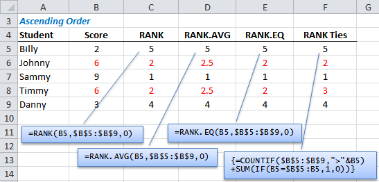
Let’s look at the different functions:
Excel RANK Function
The syntax for the RANK function is:
=RANK(number,ref,[order])
Number: this is the number you want to rank.
Ref: this is the list of numbers you want your ‘number’ compared to.
Order: this is whether you want your ranking in ascending order or descending order. Use 1 for descending or 0 or omit the value for ascending.
Excel RANK Function Limitations
One of the problems (or benefits depending on your needs) is with ties.
If there are duplicate values in your list they will be given the same rank, as you can see in column C above there are two values with a rank of 2.
Also notice that the 3rd place is skipped because there are two 2nd rankings.
Excel RANK Tie Break - Method 1
There are several different formula options to avoid the tie break situation we have above. Most of them use a similar approach but I think this is the most elegant.
In column F below you can see the tie between Johnny and Timmy is now resolved.
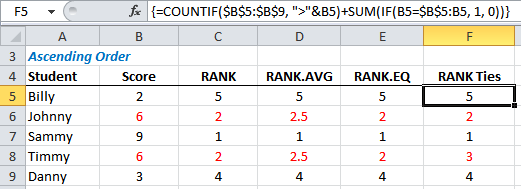
I’ve used an Array formula to resolve the tie break. Notice it doesn’t even use the RANK function.
Our formula in cell F5 is:
=COUNTIF($B$5:$B$9, ">"&B5)+SUM(IF(B5=$B$5:B5, 1, 0))
Since this is an array formula you need to press CTRL+SHIFT+ENTER to enter the formula which will have Excel put the curly brackets in for you {see formula bar in image above}.
The COUNTIF part of the formula counts how many other numbers there are in the list that are greater than the number you are ranking. So in this example there are 4 other values greater than 2.
The SUM part of the formula counts how many occurrences of 2 are in the range B5:B5.
Huh, that's only one cell.
Yes but as you move down the column the range increases. So by cell F7 the range we are comparing to is $B$5:B7, hence the absolute reference is only applied to B5.
The result of the two parts of the formula is:
=4+1
Hence the rank of 5.
In the event of a tie break the order of the duplicate numbers determines which number is ranked 2nd vs 3rd etc.
In this example Johnny’s score is higher up the list than Timmy’s and therefore is awarded a rank of 2, with Timmy getting 3 because he is below Johnny in the list.
Whilst this may seem a bit crude (and unfortunate for Timmy), most tie break solutions use order to solve a tie break.
Excel RANK Tie Break - Method 2
One alternative is to use another metric to generate a unique score. But this means you have to be measuring something else other than the score.
Let’s say you also track time.
You could then use the time metric, divided by a large number, say 100,000, then multiplied by the score to generate a new, unique score that’s slightly lower than the original like in the example below (see formula in formula bar).

You can see in the above example Johnny has a time of 30 and Timmy a time of 20, with the lower time being better.
We can then first determine whether the score is a duplicate using the COUNTIF function.
If it is we then adjust the score by multiplying it by the time in column H, divided by a large number (so that we only adjust the score slightly).
If it's not a duplicate we can simply keep the score.
The result is a new score for Johnny of 5.9997 and for Timmy 5.9998.
We can then go ahead and use either RANK or RANK.EQ with less chance of dupliates.
Of course if Johnny and Timmy also got the same times then we'd still have duplicates.
Excel RANK in Descending Order
To flip the order to descending simply enter a 1 as the argument for [order].
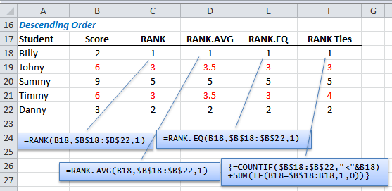
Ranking Tie Breaks in Descending Order
It’s easy to change the order of the tie break ranking by changing the greater than sign to a less than sign like this:
=COUNTIF($B$5:$B$9, "<"&B5)+SUM(IF(B5=$B$5:B5, 1, 0))
Excel RANK.AVG Function
The RANK.AVG Function is new in Excel 2010 and it was intended to create an alternative to duplicate ranks. The syntax is the same as RANK.
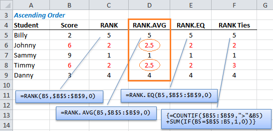
It still compares the number to its position in the list and it skips values. Behind the scenes it gives each duplicate a rank, and then finds the average for them.
For example Johnny would be given a rank of 2 and Timmy a rank of 3 with the average being 2.5.
If there were three students with a score of 6 it would give them the ranks (2 + 3 + 4)/3 and return a rank of 3 and would skip ranks 2 and 4.
Excel RANK.EQ Function
Again the syntax is the same as RANK.
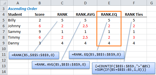
The RANK.EQ function returns the rank of a number in a list of values. If more than one value has the same rank, the top rank is returned.
This is exactly the same as the RANK function but since RANK plain vanilla will be decommissioned eventually it's wise to use RANK.EQ if you have Excel 2010 or later.
Finding 1st, 2nd and 3rd Student Names
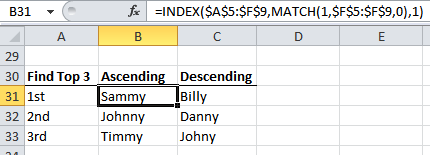
Use an INDEX and MATCH formula to find the names of the students ranked 1st, 2nd and 3rd.
If you monitor sports results, or student scores like the examples above then the RANK function may come in handy.
What do you use the RANK function for? Let me know in the comments below.
Excel RANK Tie Break – Method 1
I just tried using the array formula you suggested in lieu of Rank. Everything seemed to be going fine until I ran into and issue where I still got a duplicate ranking even though the numbers are no where the same.
Formulas: COUNTIF($AA$114:$AA$164,”>”&AA146)+SUM(IF(AA146=$AA$114:AA146,1,0))
COUNTIF($AA$114:$AA$164,”>”&AA157)+SUM(IF(AA157=$AA$114:AA157,1,0))
Values: AA146 = 8.86% Rank = 7
AA157 = 8.90% Rank = 7
Please I need help with this. I can’t figure out what the issue is.
Thanks
Hi,
I tested with your values and formulas, but I get different ranks. Can you please upload a sample file on our forum, to see what happens?
Still trying to figure that out, but the other issue I am running into is that the formula only seem to RANK descending. Is there an option to restructure the formula to RANK Ascending?
Can you please upload a sample file on our forum? Hard to see what happens without data.
I’m trying to write a formula in summary f5 that can be copied down to summary f14 to determine true or false of the corresponding marshmallow costs of all marshmallows. I dont know how to write the formula. Do I use MIN OR RANK.EQ?
Hi Natasha,
The question isn’t clear enough to provide an answer and without seeing your data it makes it more difficult.
What is ‘summary’ ? A worksheet?
What criteria are you using to determine if the costs are true or false? What does this represent?
Please start a topic on the forum and attach your workbook.
Regards
Phil
thanks, for this chance to a write acomment,
im try to do my final roster using excel, whant i got rank, when i calculated the rank of the srudent it done 1st, 2nd but what make mw wrong on the Avarge rank,.so, how can calculated b/c if the student ranked 1st in first simster and rank10th in 2nd simister, what is the avarage of rank among the whole atusenta.
thanks,
john
Hi Yohanes,
Please post your qs on the forum and supply your workbook.
Regards
Phil
Nice
I do reporting in a call center, and we need to know the agent rankings for several different metrics. Since they work as teams, what we would like to do is rank each individual on each team, and then show their rank compared with everyone. Is there a way to use the rank.eq function on several different selections, or must they all be contiguous?
Hi Mark,
RANK.EQ requires a contiguous range of cells. You’d be best to rearrange your source data to suit the ranking. From there you can derive your different metrics.
Mynda
Using Countif to Rank & Index, Match to find 1st, 2nd is wonderful idea,, ☺
Glad you liked it, Rajesh 🙂
Hi,
im using old excel and don’t have the rank.ave function, is there an alternative formula to obtain same result as rank.ave function?
Grade Rank
88 5
89 4
90 2.5
90 2.5
91 1
Thanks
regards,
mel
Hi,
Considering that your data is in range A2:A6, the following formula will return the same result as Rank.AVE function:
Note that this is an array formula, make sure you press Ctrl+Shift+Enter keys after editing the formula.
If you do not want to use an array formula, you can try this version:
Cheers,
Catalin
Wow thank you so much Catalin, i got same result as rank.ave function =) using the sumproduct formula.
one more thing if it is not to much to ask, how can i reversed the order from descending to ascending.
regards
Hi,
You can try this version, using the old Rank:
– descending:
– ascending:
Cheers,
Catalin
Indeed it is unfortunate for Timmy 🙂
If ties were okay, you can do this,
In Cell G5, enter =IF(COUNTIF($B$5:B5,B5)>1,””,B5) and copy down to Cell G9 to hide duplicates.
Then enter =RANK(B5,$G$5:$G$9) in Cell H5 and copy down to Cell H9.
This way you can see true, and fair, rank. (Hope I got the cell references right!)
We use RANK or RANK.EQ to find out the order or position in a list of scores or ages or any values, otherwise to know who is the 1st, the 2nd..etc.
But still I want to know are these two functions exactly the same or there may be some difference between them?
Thank you for the tutorial and thank you if you answer me.
Hi Rbi,
RANK.EQ was introduced in Excel 2010 when the new RANK.AVG was added. RANK.EQ is exactly the same as RANK but since RANK will eventually be decommissioned it’s a good idea to use RANK.EQ going forward.
Mynda
Rank should be like this
Score Rank
9 2
5 3
3 4
5 3
10 1
2 5
I am not getting this type of rank. Can anybody calculate like above.
Thank
Hi Muhammad,
Try Descending – 0 for your Order Argument, like this:
Cheers.
CarloE
That doesn’t really fix it does it…
How can there not be a simple way of choosing to do like below just in the Rank function? Or is there?
Values Standard Rank “Absolute Rank”
9 2 2
5 3 3
3 5 *4*
5 3 3
10 1 1
2 6 *5*
Any other smart way of doing it?
Regards
M
Hi Mathias,
You can try an upgrade to RANK function, that will return unique results, even if we have duplicate values in range.
Considering that the range of values is in A1:A20, try this formula in B1 copied down:
=RANK(A1,$A$1:$A$20)+COUNTIF($A$1:A1,A1)-1
Or this one, which seems to be what you are looking for:
=SUMPRODUCT(–(A$1:A$20>A1)/COUNTIF(A$1:A$20,A$1:A$20))+1
Catalin
I need RANK like this:
Score Rank Want this
10 7 4
20 1 1
15 6 3
10 7 4
18 3 2
20 1 1
18 3 2
18 3 2
Thanks
Hi Fida,
Try this formula then (with your data in A2:A9):
=SUMPRODUCT(–(A$2:A$9>A2)/COUNTIF(A$2:A$9,A$2:A$9))+1
Cheers,
Catalin
hi i have a similar problem to this, im using excel 2010 and trying to adapt an old excel workbook for our snooker league, the league table is calculated intially by point scored and if that is tied then the next criteria would be the lowest points scored against, if still tied then lowest games lost is used.
column m4:m27 is points scored, K4:k27 is points against and I4:I27 is games lost.
the ranking at the moment only does it by points scored using =rank(m4,$m$4:$m$27) etc is there a way i can get the other criterias added if this is a tie, id appreciate any help you can offer.
Hi Nigel,
I have actually a solution for this but It might take long or to be more accurate, complicated to explain it here.
So why don’t you send your file to me via help desk.
Please do clarify how are we going to rank the other criteria. To be honest, We need some VBA on this one.
Cheers.
CarloE
many thanks for the answer i was beginning to think vba might be needed as anything i tried i was jsut going round in circles using rank etc, file is quite big but ill attempt to send,many thanks
Hi Nigel,
You don’t need to send everything. Just a file with a few examples and your explanations.
HELP DESK here.
CHeers.
CarloE
Need to rank a column of numbers including ties but want the rank following a tie to be the next consequtive Rank number up and not skip Rank numbers. For example: dataset (50,80,60,60,40) would be ranked (4,1,2,2,5) but I need it returned as (3,1,2,2,4)…after the ranking of 2, the next consequtive Rank number should 3, not skip to 4.
Thanks for any help!!!!!!!
Hi Adam,
You can use this formula:
Hi Mynda,
I am VERY green with excel, but I am trying to figure things out….
PROBLEM: I am trying to keep track of winners in a football pool. I have 6 people that play each week, and I need to know the winner each week by:
a) the person with the most wins that week or,
b) if it’s a tie, then the person with the closest combined score wins. (The combined closest score is the combined score of the two teams playing during the Monday Night Football game (eg. someone tells me their combined predicted score is 38 (Dallas=17, Chicago=21 for a total combined score of 38) while someone else tells me their combined predicted score is 46. The ACTUAL score for that Monday Night Football game is 43. The person who guessed 46 is closer than the person who guessed 38)
I have the closest score formula figured out, and the result displayed in a separate cell using an array formula.
I also have the max number of wins figured out and the result displayed in a separate cell using a simple MAX function.
I EVEN have a complex match criteria function but it ONLY returns the person with BOTH the most wins AND the closest combined predicted score…I can’t seem to get it to deal with a circumstance of a TIE with the most wins.
Does this make sense?
Can the RANK function somehow help me to break the tie of the most wins first, and then return the winner with the closest combined predicted score?
Thanks,
Rod
P.S. I am using Excel 2003
Hi Rod,
Since you only have Excel 2003 then you can’t use the RANK function to solve a tie break. You have to use either order of values (the value first in the list gets priority), or another factor to generate a unique value to then rank as in the COUNTIF/SUMIF example above.
If you’d like to send me your Excel file I can take a look and give you a more tailored solution.
Kind regards,
Mynda.
it great
Cheers, Kingsley 🙂
Hi,
This is a great help, I use Ranks within my daily reports as our managers like to see a performance table.
May I kindly ask if you do have a “Rank Ties” formula that looks also to a 3 condition… i.e. Location, Date, Name, Score.
I would appreciate the help.
Kind regards,
Hi Vitor,
Glad you found this useful. I’m not sure how you’d use location and name data in a ranking scenario. If the other conditions were values you could multiply them by one another to get a unique value and then find the rank of your new unique value.
Can you please give me a more specific example?
Kind regards,
Mynda.