The options in the Pivot Chart library are limited, which you’ll know if you’ve ever tried to create a Scatter chart. Last week we looked at a workaround to create a scatter chart from a PivotTable, which is great if you want to use Slicers. However, we can also create an Excel Power Query Pivot Chart. Strictly speaking it’s a regular chart based on data pivoted in Power Query.
Yes, Power Query can pivot data too and the benefit of this approach is that when your source data gets updated you can refresh the query or set it to auto-refresh.
Power Query Pivot Chart Example
Below is a snapshot of my source data. Notice it’s in a tabular format ready to pivot (this is key):
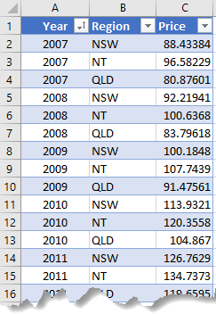
To plot the data above in a line chart I used Power Query to pivot the data with the regions across the columns and years down the rows, like so:
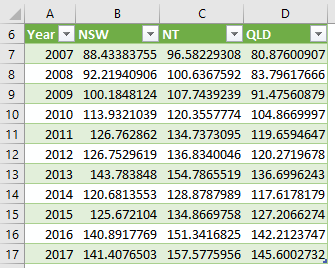
From this table I can insert a regular chart:
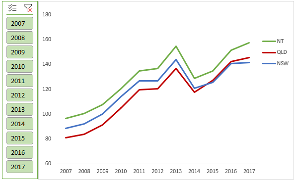
Tip: Power Query tables can be used to insert any chart type, unlike PivotTables, which have a limited library of Pivot Charts.
Limitation: Slicers for Tables are only available for the X axis and in Excel 2013 onward. If you also need Slicers for the row labels/Ledgend Entries then try the regular chart from a PivotTable technique described here.
Building a Power Query Pivot Chart
It’s super easy to pivot data with Power Query.
Step 1: Select your source data and press CTRL+T to format your data in an Excel Table (you don’t have to do this, but it makes it easier).
Step 2: Excel 2016 onward; go to the Data tab > From Table/Range:
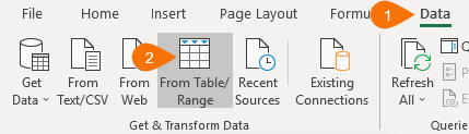
In earlier versions of Excel go to the dedicated Power Query tab > From Table.
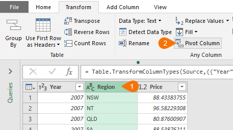
Step 3: Select the column containing the data you want to pivot across the columns, in my case it's the Region column > Transform tab > Pivot Column:
Step 4: Select the Values Column, in this example it’s ‘Price’, and aggregation type in the dialog box:
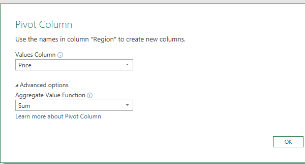
Tip: You can aggregate by average, count, minimum, maximum and more
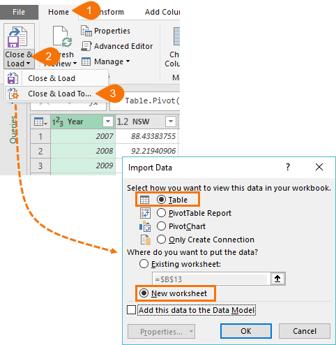
Step 5: You’re ready to load the data into the worksheet. Home tab > Close & Load > Close & Load To. Then in the Import Dialog box load it to a Table in a New worksheet:
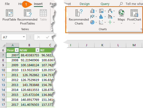
Step 6: Your pivoted query data is ready to plot in a chart.
Updating your Excel Power Query Pivot Chart
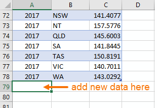
When you get new data, simply add it to the bottom of your source data table:
Then right-click the Query table > Refresh:
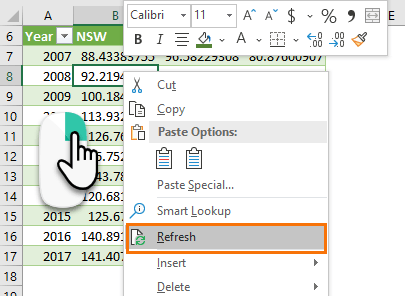
The chart will now be updated.
Power Query Auto Refresh Options
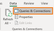
You can set the query to refresh upon opening the workbook or at set intervals. To do this open the Queries Pane (Data tab in Excel 2016 onward, or Power Query tab in earlier versions):
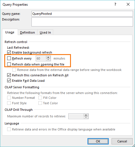
Right-click the query in the Queries & Connections pane > Properties:
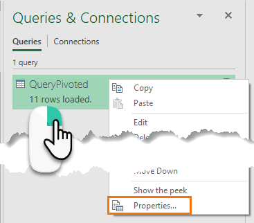
In the Query Properties you’ll find the refresh options:
More Power Query
I can’t say enough good things about Power Query. I’m not exaggerating when I say the efficiency gains from Power Query can be life changing.
If you’d like to learn more check our past Power Query tutorials here.
And if you want to master Power Query, please consider my Power Query course.
Download the Workbook
Enter your email address below to download the sample workbook.
Please Share
If you liked this please click the buttons below to share.


Hi,
I have two seperate sheets of sales data for 2 years, each of which has around 8 lacs rows.
I want to connect two pivot tables from these two sheets with one slicer only.
Please help.
Hi Sarvesh,
As this data is the same information, albeit for 2 separate years, you must consolidate this data into a single table. It won’t make sense to keep it as two separate tables. You can use Power Query to append the data in separate sheets.
Mynda
Hi Mynda, I always appreciate your tutorials so thank you for sharing.
Thanks, Mehdi! Great to know.
Great article, thanks.
However I have updated the data in the source table and then refreshed the Pivot Table that is linked to Power Query and the associated chart does not update.
I have to right-click on the chart and select ‘refresh’.
How do I make the chart update when the pivot table is updated?
cheers,
Martin
Hi Martin,
If you right-click on the chart and there is a ‘Refresh’ option then you have yourself a Pivot Chart, not a regular chart, which is what I’ve used in this tutorial.
When you create a Pivot Chart from a Power Query table you have to go through two refreshes; once to refresh the query and for Power Query to load the data into the Table in the worksheet that the PivotTable and Chart reads, and another to refresh the PivotTable so it picks up the new data in the Table in the worksheet.
If you’re going to use a Pivot Chart then when you ‘Close and Load To’ you should choose PivotTable and skip loading the data to the worksheet altogether.
I hope that points you in the right direction.
Mynda
Thanks for the tutorial, Mynda. The auto-refresh is a great feature.
A comment on Step 5 for those not familiar with PQ: As a shortcut, if you know you want the data loaded into a new spreadsheet, you can just select “Close and Load” rather than “Close and Load To” and avoid a few extra steps, as that will always load to a new worksheet for a new query. Downside of this is that if you get into the habit of doing this vs “Close and Load To”, you miss the option to just create a connnection in memory.
You’re welcome, Glenn. Thanks for sharing your tip. Just note though that Close and Load will only load to a table in a new sheet if you have that set as the default. By default it is, but that doesn’t mean someone hasn’t changed it, which is why I tend to show all of the steps.
Great remark Mynda as, in my case, I configured PQ to just create a connexion to the data
Glad you found that useful. I prefer this too.
I want to thank you for you generosity in sharing content and practice worksheets. It makes a difference for my own learning.
It’s my pleasure, Alberto. It’s great to know I can help.
Excellent tutorial, Mynda, very easy to follow. Thank you very much for always sharing awesome tips, it’s a pleasure to read your posts every week 🙂 I am impressed what can be achieved with Power Query, it’s a life changer
Thanks, Juan. Great to hear you’re loving Power Query. Spread the word about it to your colleagues 🙂