Excel PivotTable Named Sets enable you to pick and choose which columns or rows you want included in your PivotTable report, but there's a catch. They require you to use Power Pivot to create your PivotTable. Don't worry, it's so easy you won't even realise you're using Power Pivot.
Note: Named Sets are only available in Excel 2010 (with the free Power Pivot Add-in), or Excel 2013 where you have a version that includes Power Pivot.
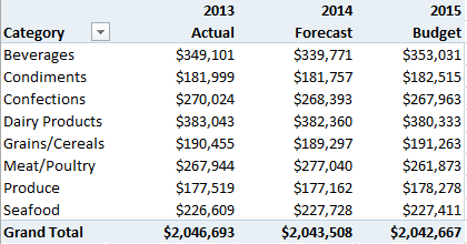
For example let’s say you are preparing budget, forecast and actual reports spanning multiple years and you have the following data:
- 2013 actual and budgeted sales
- 2014 actual, forecast and budgeted sales
- 2015 budgeted sales
You’d like your PivotTable report to look like this:
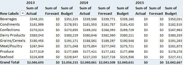
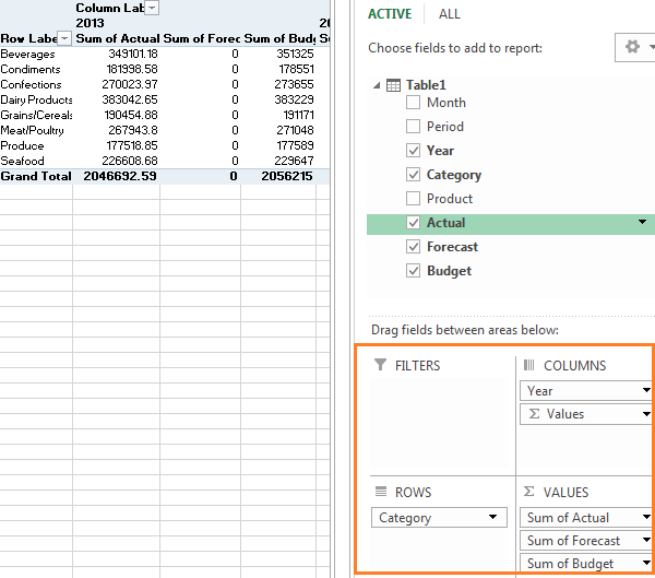
But a regular PivotTable looks like the one below with columns for Actual, Forecast and Budget for every year. Ugh, annoying:
We want to get rid of the unwanted columns:
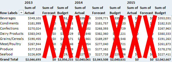
The only choice we have, if you don’t want to resort to formulas, is to hide the columns you don’t want, but that’s a bit laborious, not to mention deadly if you’re showing grand totals and they don't add up. Yes ‘deadly’…. your boss may kill you if he/she makes decisions based on that report. Who said accounting was boring? It's life and death stuff!.
However, in Excel 2010 and 2013 it’s easy with Named Sets.
Enter your email address below to download the sample workbook.
Creating Named Sets in Excel
In Excel 2013 it’s pretty straight forward (you don’t even need to know how to use Power Pivot). Let me show you:
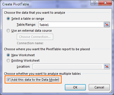
Step 1 Excel 2013: Insert a PivotTable and at the Create PivotTable dialog box check the ‘Add this data to the Data Model’ check box (tip: the ‘Data Model’ is Excel 2013 speak for ‘Power Pivot’):
In Excel 2010 it’s a bit more involved:
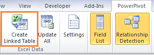
Step 1 Excel 2010: Select your data > go to the PowerPivot tab > click on the ‘Create Linked Table’ button.
Step 2 Excel 2013: Create your PivotTable (Insert tab > PivotTable) bring in all the fields you need (it’ll be ugly at first but stick with me):
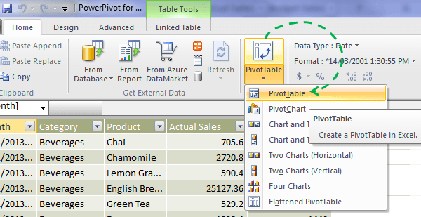
Step 2 Excel 2010: In the Power Pivot window > Home tab > PivotTable > PivotTable:
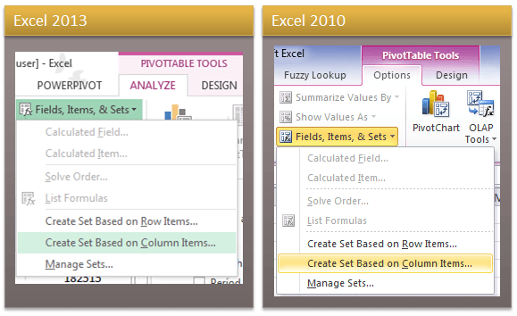
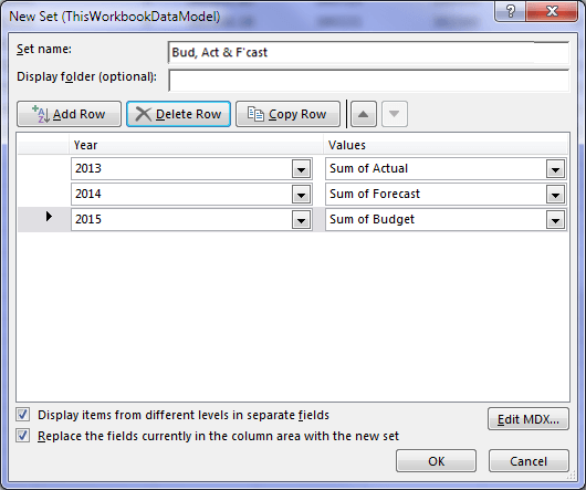
Step 3: Create the Named Set by selecting any cell in the PivotTable > PivotTable Tools: Analyze tab/Options tab > Fields, Items & Sets > Create Set Based on Column Items:
Step 4: In the New Set dialog box (1) give your set a name, (2) click beside the fields you don’t want in your report (a blue background will appear to show which field is selected), (3) click the Delete Row button to remove them:

When you’re done removing the fields you don’t want your New Set dialog box looks like this:
And once you click OK, your PivotTable will look like this:
Notice in the PivotTable Field List that you have a new field called ‘Sets’:
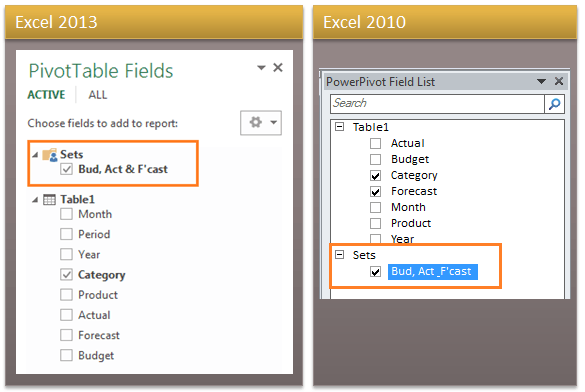
This field can be added to any PivotTables you create which share the same source data and Pivot cache. Nice.
Other uses for Named Sets
Create groupings of regions/departments for specific salespeople or department managers. Heck, any grouping you want.
In the example above we created groupings based on Column items but you can also create groupings of Row Items.
Things to know about Named Sets
- What you may not have realised (particularly in Excel 2013) is that you have actually created a Power Pivot model, and the PivotTable you created with the Named Sets is in fact a Power Pivot PivotTable.
- In Power Pivot you cannot group dates so you’ll notice in my file that I have inserted a column for the Year field.
- Once you have added your fields to a Named Set and you’re using that named set in your PivotTable, you cannot add any of the fields to your PivotTable a second time.
BTW, Power Pivot is now officially two words however it is still written as one in the Excel Ribbon for Excel 2013.
Want More?
If you liked Named Sets why not look at what else Power Pivot has to offer. See a demonstration of Power Pivot in action and check out my Power Pivot course here.

I have a really strange problem – I created 5 pivot table sets, but only 2 appear in the pivot table field list “Sets” folder. How can I solve this?
Not sure, sorry. I’ve not experienced that problem before. If you want to post your question on our Excel forum where you can also upload your file and we can help you further.
Hi! Thanks for the tips. I was looking into expanding more the named data sets, but couldn’t find how far can you go with mdx functions inside of them. For example, trying to use the sum function, always threw an error, but the filter one, did work. Do you know where can I find more information on how to use mdx inside Excel with a simple Power Pivot data model?
Thanks again!!
Hi Ricardo,
Sorry, MDX is not my specialty. However, I found this page that might give you the answers you’re after.
Mynda
It seems there is a problem to download either the 2010 or 2013 workbooks….The links do not work.
Anyway : Simply the BEST !!! THANK YOU !!! This is the absolutely the best Excel examples and tricks I ever discovered. There absolutely nothing equivalent in France ;-(( but we are an “old” country, isn’t it ??
Hi Nikky,
Thanks for your kind words. I’m delighted you’re enjoying our tutorials.
In regards to the workbooks, please right-click the download links and then choose ‘save as’ to download them.
Please let me know if you have any problems.
Kind regards,
Mynda
Hi Nikky,
Glad to hear that you found our website useful 🙂
Try to right click the files and select: Save Target As, instead of clicking the link, it might open the excel file in browser instead of downloading it. Even so, if the excel is opened in browser, use the browser menu and save the page as an xlsx file on your computer.
Cheers,
Catalin
Mynda,
thanks a lot!!! And Paul – I had the same problem, so Mynda and Paul – thanks a lot to both of you!!!
Malina
Glad we could help, Malina 🙂
Hi Mynda,
I am having a problem creating variances and a named set. If I have, say, data for 2013, 2014 and 2015, I can create a variance using “Difference from previous”. This works fine but, obviously, gives a blank column(s) for the first year.
If I try to create a named set excluding that blank column then the pivot table goes back to base SUM totals and loses the Difference from function.
I hope that makes sense. Is there a way around this?
Kind regards.
Paul
Hi Paul,
The Difference From setting requires the data to be present in the pivotTable for it to calculate. If you remove 2013 from your set it will revert to the default SUM setting (as you know) and then if you change the field back to ‘Difference From’ again it will simply show zero in 2014 because 2013 isn’t present.
Said a different way: This is because the values area of a PivotTable works in context of the row and column labels. If you remove the column label for 2013 then it doesn’t know what was ‘previous’ as that label is no longer in the PivotTable.
Alternatively you can write a custom DAX measure using the PREVIOUSYEAR function, or the simplest option is to hide the 2013 column!
Kind regards,
Mynda
Hi Mynda,
Thank you for that explanation. An “of course” moment!
“…or the simplest option is to hide the 2013 column”. Aaargh – why do I not think of the obvious. 🙂
Many thanks.
Paul
🙂 you’re welcome, Paul. I’m just glad one of the options was viable.
Hi,Dear Mynda
Really useful, thank you very much
kind regard
Thanks, Mano. Glad you’ll find it handy.
Mynda
Crazy powerful. This will clean up several reports nicely. Thanks for sharing.
Hi Jef,
Yes, it’s like a hidden gem! Glad you’ll find it useful.
Mynda
Really useful, thanks
Cheers, Mike 🙂
This is very useful! Did I miss something, or how did you change the column headers from “Sum of Actual” (etc.) to “Actual”? Thanks.
Hi Dena,
Glad you liked it. You can just type over the ‘Sum of Actual’ with Actual with a space at the beginning or end to differentiate it from the column name 🙂
Mynda
Thanks Mynda – I did not know that either! Sounds easy enough.
Dena
You’re welcome 🙂
Superb! Why didn’t we know this before???
Thanks guys,
Excellent learning….
Adi
Thanks, Adi 🙂
Better late than never!