Excel PivotTable Show Values As

The Excel PivotTable Show Values As menu has a load of handy instant calculations you can use. For example you can choose to show the values as:

• Percentages of the row, column or grand totals
• The difference from or % difference from
• Running totals
• Ranking
• And index

Kevin emailed me with a vehicle log book and he wanted to calculate the distance of each trip. It’s pretty complicated with formulas but with the PivotTable Show Values As tool it’s a doddle. Let’s take a look.

Excel PivotTable Show Values As Example

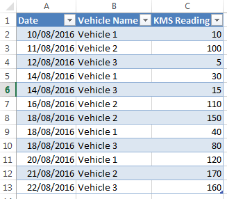
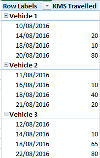
Let’s say you have a list of vehicles and you record the odometer reading at the end of each trip like so:

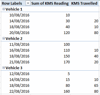
From this data I can create the PivotTable below using the Show Values As > Difference From > Base Field: Date, Base Item: Previous, to calculate the KMS Travelled shown in the third column:

Steps to build this PivotTable

Step 1: Insert a PivotTable

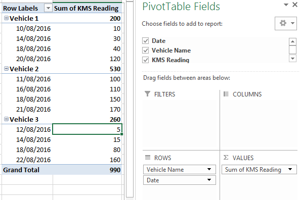
Step 2: Drag the KMS Reading column to the values area again so you have it in the PivotTable twice:

Step 3: right-click the Sum of KMS Reading2 column > Show Values As > Difference From:

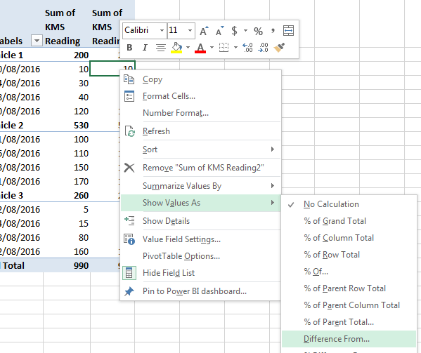
Note: in Excel 2007 you'll find the Show Values As menu in the Value Field Settings > Show values as tab.

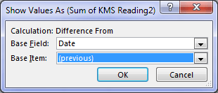
In the Calculation Difference From menu choose Base Field: Date and Base Item: (previous):

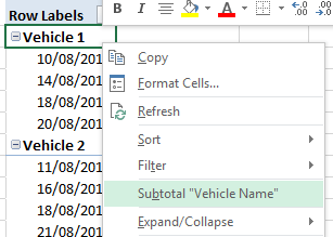
Step 4: Remove up the subtotals for the vehicles; right-click Vehicle 1 > deselect ‘Subtotal “Vehicle Name”. And remove the Grand Total; right-click Grand Total>‘Remove Grand Total’.

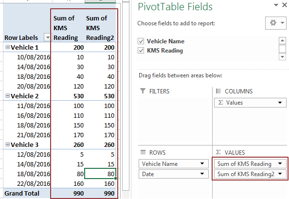
Step 5: Give the ‘Sum of KMS Reading2’ column a new name; simply type over the header cell with a new name. Just make sure it’s different to any of the existing source data column names:

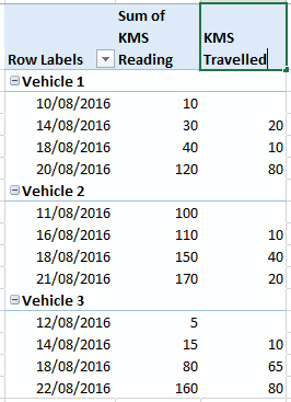
So you can see it’s pretty easy to calculate the difference from one odometer reading to the next using Show Values As.

Let’s look at some other things we can do.

Excel PivotTable Show Values As Examples

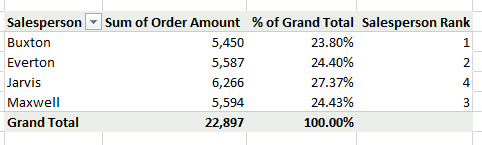
The PivotTable below uses Show Values As to display the % of Grand Total (for the Order Amount) and Sales Person Rank (based on Order Amount) in ascending order:

And if we add another grouping for the countries the % of Grand Total adapts, as you can see below.

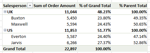
In the image above the last column, the % of Parent Total, calculates the % Order Amount within each country.

Also, in the examples above I’ve left the Sum of Order Amount columns in the PivotTables for reference, but you can remove them if you prefer to just see the result of the Show Values As fields. For example, in the log book analysis you might only want to see the KMS travelled like so:

More Show Values As

A while back I wrote a tutorial on how to use Show Values As to calculate the year on year change.

Download the workbook and try it yourself

There are loads of ways you can use the PivotTable Show Values As tool so download the workbook below and have a play around with it.

Thanks

Thanks to Kevin for asking the vehicle log book question which prompted me to write about this topic.

Have you got a favourite use for Show Values As? Please share it in the comments below.