Excel PivotTable Percentage Change

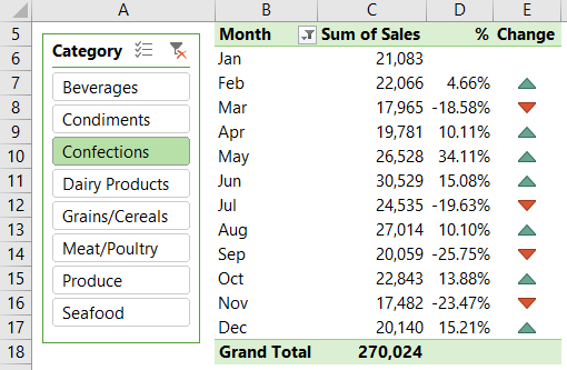
PivotTables can make quick work of summarising and analysing data and they have some handy built in percentage calculations available via the Show Values As menu.

The Excel PivotTable Percentage Change calculation is achieved with the % Difference From option and is useful for quickly identifying if this month/quarter/year is better or worse than last month/quarter/year.

Add in some Conditional Formatting to your PivotTable, and throw in a Slicer and we’ve got a super quick, visually appealing, interactive report at the click of a few buttons.

Let’s look at how to build the month on month percentage change PivotTable above and watch the video to learn what NOT to do when calculating the percentage change from zero.

Download the Workbook

Watch the Video

Excel PivotTable Percentage Change

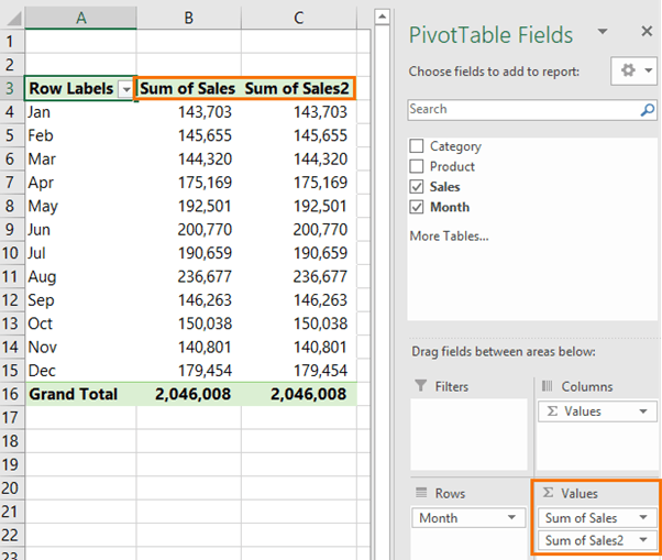
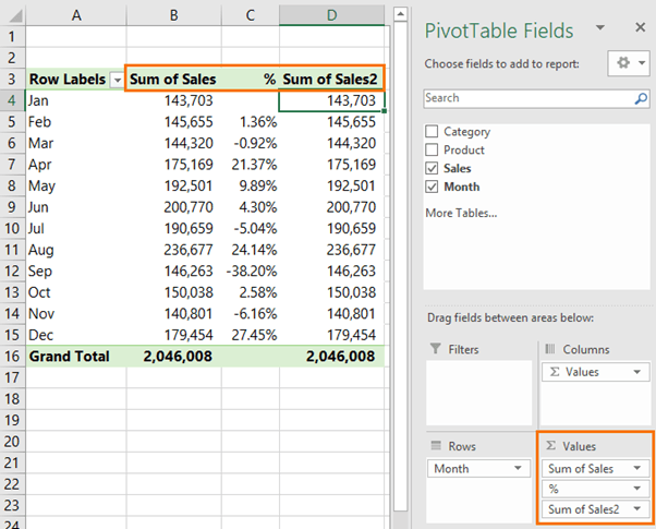
Step 1: Start with a regular PivotTable, and add the field you want the percentage change calculation based on, to the values area twice:

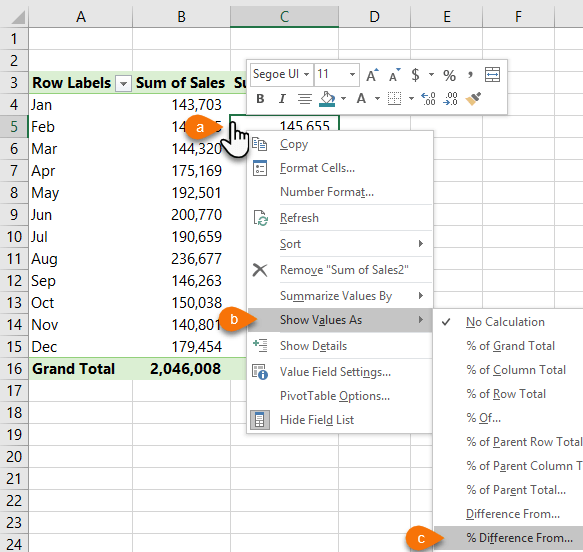
Step 2: Right-click any values cell in the Sum of Sales2 column > select Show Values As > % Difference From…:

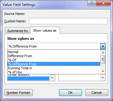
Note to Excel 2007 users: The Show Values As options are in the Value Field Settings dialog box:

Tip: You don’t need the Sales field in the Values area twice to show the % Difference From. If you only want to show the percentage change and not the actual Sales amounts, then you can simply add the ‘Sales’ field to the Values area once and then set that field to % Difference From.. via the ‘Show values as…’ menu.

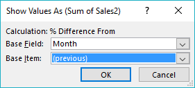
Step 3: In the Show Values As dialog box set the Base field to Month and the Base item to (previous):

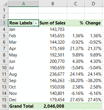
Your PivotTable should now look like this:

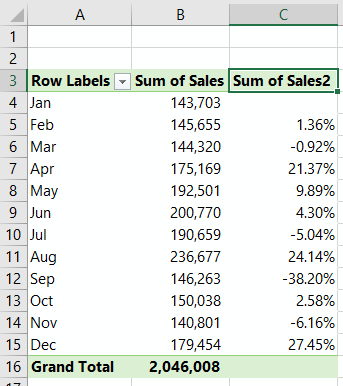
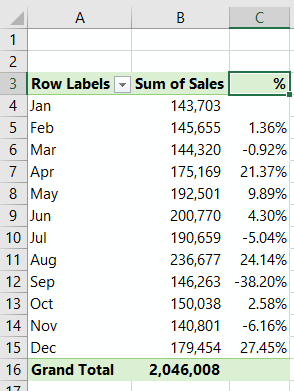
Tip: Give the ‘Sum of Sales2’ field a better name. Simply type a new name in cell C3, making sure it’s not the same as any of the field names in your PivotTable source data. I’ll just call mine %. You’ll see why in a moment:

Add some Conditional Formatting

We can make the % change percentages easier to read with some Conditional Formatting visual indicators. I like to place these in a separate column, but if you’re happy for them to share column C then you can skip steps 4 and 5.

Step 4: For this we’ll need to add the ‘Sales’ field to the Values area again:

Step 5: Right-click the Sum of Sales2 column > Show Values As > % Difference From, and then same as before; Base field is Month and Base item is Previous.

Also give the column a new name. I’ll call mine ‘Change’, as you can see below:

Step 6: With any cell in the ‘Change’ column values area selected, go to the Home tab > Conditional Formatting > Icon sets. Here you can choose from different icons, but I’ll stick with the directional triangles:

This will apply the formatting to the selected cell.

Step 7: To apply the formatting to the whole ‘Change’ column, click the drop down beside the cell and select ‘All cells showing “Change” values for “Month”, as shown below: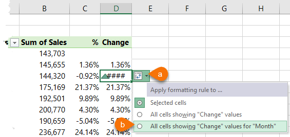

It should now look like this:

Notice that there are some neutral/yellow icons. We want to change the formatting to simply show green up triangles for positive change and red down triangles for negative change.

Step 8: With any cell in the ‘Change’ column selected, go to the Home tab > Conditional Formatting > Manage Rules. This opens the Conditional Formatting Rule Manager dialog box (shown below). Select the icon set rule and click ‘Edit Rule’.

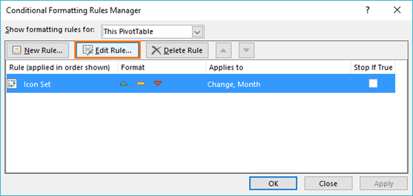
Tip: You can also double click the rule to open the rule editor window, shown below:

Edit the settings as shown in the image below. Note: I’m choosing to only show the icon in this column because column C already has the percentages displayed.

Your PivotTable should now look like this:

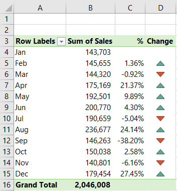
Tip: I’ve centered the Conditional Formatting icons using the cell alignment on the Home tab.

For the icing on top, add a Slicer and allow your user to interact with the PivotTable, as I’ve done for the Category field:

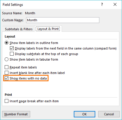
Tip: Just in case some months don’t have any data, I’ve set my Month Field settings to ‘show values with no data’ to ensure all months are listed:

Note: Months with no data will result in a #NULL! error for the % Difference From calculation. It’s not an issue here, but something to be aware of if you see #NULL! errors in your PivotTables.

Handling Errors in PivotTables

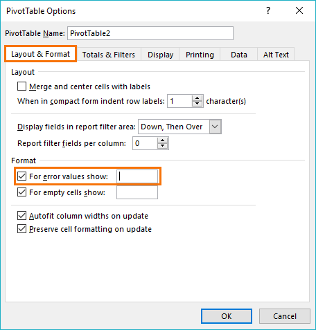
Now, obviously we don’t want our PivotTables littered with errors, especially if we’re presenting them in a report, that would just create unnecessary questions and we’re busy enough.

Thankfully we can supress errors in the PivotTable options; right-click the PivotTable > PivotTable Options > on the Layout & Format tab check the ‘For error values show’:

Want More?

Discover more PivotTable tutorials here, or take our PivotTable course.