Excel PivotTable Month Comparison [Video]

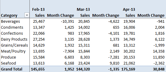
In this last tutorial, in my 3 part series on PivotTable tips and tricks, I’m going to show you how to include the month on month change. In the example below we can see that beverage sales in Feb were $10,391 less than the previous month, and in March they were $4,622 less than February:

Watch the Video

For best viewing watch the video in 720p HD full screen.

Download the Workbook

Click here to download the Excel workbook (contains instructions).

Note: this is an .xlsx file. Please ensure your browser doesn’t change the file extension to a .zip file.

Written Instructions - How to Add Comparison to Previous Month

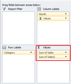
1. Add 2 'Sales' fields to the Values area like in the image below. The second one will be the difference from previous month.

2. Select any cell in the PivotTable for Sum of Sales2 and right click and select 'Value Field Settings'.

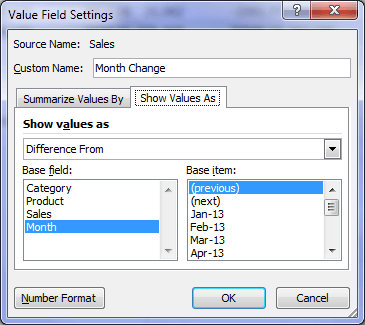
3. On the 'Show Values As' tab select 'Difference From' from the list, and choose 'Month' from the Base Field, and '(previous)' from the Base item, like this:

More PivotTable Tutorials

Click this link for more on Excel PivotTables

Do you want more like this?

Let me know by sharing this tutorial on Facebook, Twitter, LinkedIn or +1 on Google by clicking the icons below, or leave a comment and tell me what other tutorials you'd like.