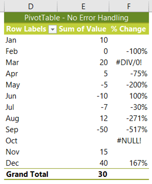
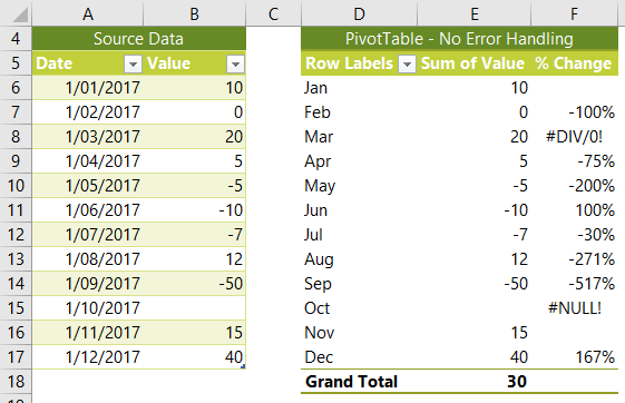
Obviously, we don’t want our PivotTables littered with #DIV/0! and #NULL! errors if we’re presenting them in a report (like the one below), that would just create unnecessary questions and we’re busy enough.
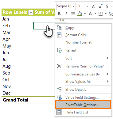
Thankfully Excel PivotTable error handling is easy to control via the PivotTable Options; right-click the PivotTable > PivotTable Options >
On the Layout & Format tab check the ‘For error values show’:
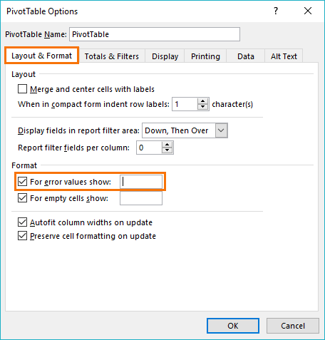
Instead of the error you can show text, like ‘N/A’, a number or leave it blank. I usually leave it blank, as you can see in the image below, because this is most likely to be suitable for all errors. Whereas if you put a value like 0 or 1, then that may not be correct in every scenario.
Types of PivotTable Errors
In the PivotTable below, column F; ‘% Change’ is a ‘Show Values As’ calculation for ‘% Difference From…’, which is uses the following formula:
=(current month – previous month) / previous month
When the ‘previous month’ is zero we get the #DIV/0! error, and when the current month has no data we get a #NULL! error, as you can see below:
#DIV/0! errors are triggered by dividing by zero. It’s the most common PivotTable error and is typically found in calculated fields or calculated items, or a calculation from the Show Values As options.
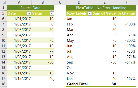
#NULL!, errors are triggered when a formula references an item that is blank. In the example above, you can see the source data for October is an empty cell (B15). You can fix this by replacing blank cells with zeros...but then you might end up with #DIV/! errors 🙂
Blanks – Notice Jan and Nov have blank results in the % Change column?
A blank is returned when the previous month is blank. And while this isn’t an error as such, some of you may prefer to see 100% or ∞, or some other value in there. After all, if you’ve gone from nothing to something (positive) then isn’t that an improvement?
Well yes, but that doesn’t mean you can represent the improvement in percentage terms.
Handling Percentage Change Where Prior Period is Zero
From time to time someone will ask me how they can override these blanks and display 100% change when the prior period was zero.
The answer to this question is always, “I’m not telling”! Not because I’m being mean, but because it would be wrong to show the percentage change from zero as 100%, or even 0%.
I don’t just leave them hanging with “I’m not telling”, I told you I’m not mean. 😉 I go on to explain why, like so:
Let’s say yesterday you had $0 and today you have $10. If you were to say that today you have 100% more $ than yesterday, then you’d be saying that you still have $0 because $0 + (100% x $0) = $0, when in reality you now have $10.
Whereas if yesterday you had $5 and today you have $10, then you can say you have 100% more $ today because $5 + (100% x $5) = $10.
In other words, you can only calculate the percentage change from ‘something’, and zero is nothing. i.e. something is a number other than zero.
So, the accepted answer when calculating the change from zero is ‘not meaningful’ or leave it blank.
And before you think you can sneak 100% in the ‘For empty cells show’ field in the PivotTable Options, I’m happy to say that won’t work for the % Difference From empty fields.
Forward this tutorial to those you know who insist the percentage change from nothing to something is 100%?
Download the Workbook
Enter your email address below to download the sample workbook.
Please Share
If you liked this please click the buttons below to share.


Thank you for the information! I am wondering if there’s a way to over ride the blanks and put in a word. I want to indicate that an item was added and put “Added” instead of blanks. Is there a way to do this, or do I have to just leave the blanks? Thanks!
Hi Erin,
Yes, just type in what you want to see instead of ‘blank’.
Mynda
Hello — working in Excel 2010 — for the pivot table, I have a column that has limited data in it. Where the column/field is blank, the pivot table displays (blank) even though I have checked the box ‘for empty cells show’ and left the input box blank. in order for the column to avoid displaying (blank), I put ‘— in the source table. What am I doing wrong? The source table will grow and I don’t want to put ‘— in manually for each new entry.
Thanks for your help.
Pat
Hi Pat,
You will see (blank) in a row label where that label is blank. The post above deals with errors in the values area of the PivotTable, not the row labels, as does the check box to ‘show empty cells as’.
If you want to avoid blanks in the row labels then you must enter something in those fields, even if it’s a space. You can do this in the PivotTable; simply select any cell containing (blank) and type a space in it. This will replace all (blank) items.
Mynda
Hi Mynda, great article as always!, quick question: With pivot tables, do you go about with calculating Variances with Negative Numbers?
For example, data pig on this article uses the function ABS() (absolute).
I been having reports with pivot tables, where variances with negatives does come right 🙁
Thanks, Carlos!
If I required more control over the calculation used for the variance I’d use a calculated field or calculated item, instead of the built in ‘Show values as…’ calculations available.
Mynda
Mynda