Excel Online PivotTables

Inserting PivotTables in Excel Online is now possible. It’s still in its infancy with many features you may be used to in the Desktop version of Excel not yet available, but it’s a start.

Inserting Excel Online PivotTables

As with any PivotTable, you need to begin with some Tabular Data. I recommend storing your data in an Excel Table so that the PivotTable can automatically pick up any new data upon refresh.

Note: Currently there’s no way to edit the source data range for your PivotTable from within Excel Online so it’s best to use Excel Tables as your PivotTable source data. If you need to edit the source data then you can open the file in the Desktop version of Excel.

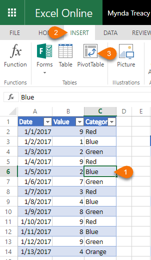
Step 1 – Select your data or any cell in your table

Step 2 – Insert tab

Step 3 – PivotTable

Step 4 – At the ‘Create PivotTable’ dialog you can edit the Table/Range detected by Excel and choose where you want to insert the PivotTable:

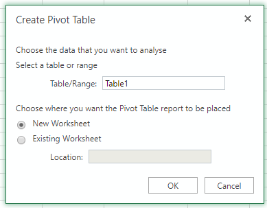
Note: Data sources are limited to data stored in the current workbook.

Step 5 – The PivotTable place holder is inserted in the worksheet grid and the Field List appears in the right-hand task pane:

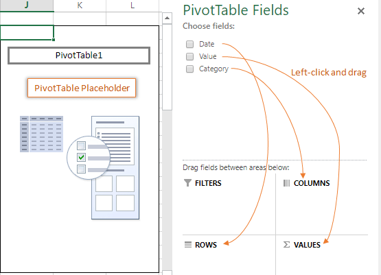
So far it looks just like PivotTables in Desktop Excel that you might be familiar with. Notice the column headers are listed in the ‘Field List’.

Place the fields in the area wells (Filters, Columns, Rows, Values); left click and drag them into place.

Hint: If you want to live on the edge just check the box for the fields and let Excel decide where to place them!

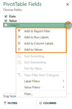
Or if you’re working on a touch screen you can click the drop down beside the field (press a field name to activate the drop-down button) and select from the menu:

And voila, one Excel Online PivotTable:

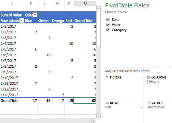
Excel Online PivotTable Tools

As I mentioned at the beginning, inserting PivotTables in Excel Online is brand new and so they don’t have the full functionality you may be used to from the Excel Desktop application. Let’s take a look at what we do have available.

Field Drop Down Menu

Clicking on a field drop-down arrow (shown below) is consistent with the Desktop version of Excel. The options differ depending on the area the field is in, with fields in the Values area also having a ‘Value Field Settings’ option:

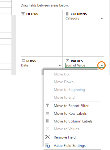
Change Aggregation Type

If you want to change a field in the Values area to Average, Count, Min or Max etc., simply click the down arrow beside the field in the field list area (image above) and select ‘Value Field Settings’. Here you can choose a different aggregation type:

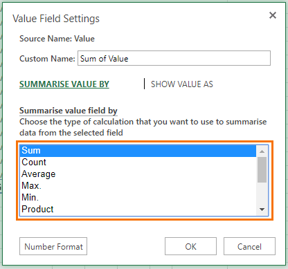
Tip: You can also give the column/row label a different name in the ‘Custom Name’ field in this dialog box.

Format Values Area

Number formats are also accessed from the Value Fields Settings menu > Number Format button. This opens the Number Format dialog shown below:

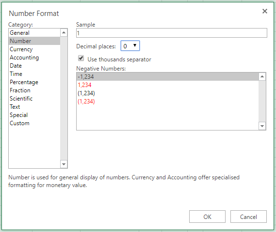
Tip: Using this dialog to set the number format ensures that as the PivotTable grows with new data those new values are formatted correctly, irrespective of any cell formatting applied, or not applied on the grid.

Show Values As

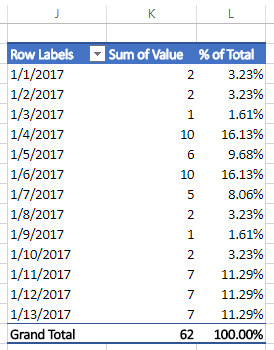
Let’s say you want to see a second column of values that displays the percentage of the total, as shown in column L below:

It’s easy done in Excel Online PivotTables:

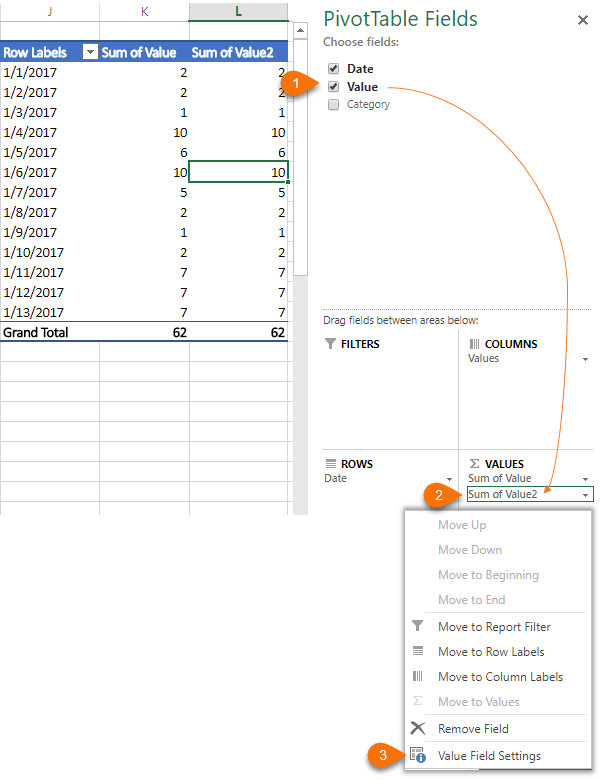
1. Add a second instance of the ‘Value’ field to the Values area
2. Click on the drop down beside the new field

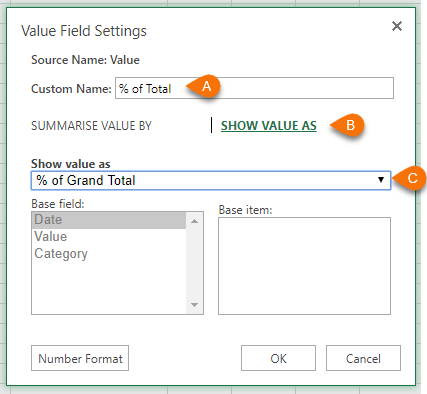
3. Value Field Settings > in the dialog box that opens (shown below):
   • A. Give your field a new name
   • B. Click the ‘Show Values As’ tab
   • C. Choose the type of calculation you want. Options from here differ depending on the calculations chosen.

Learn more about Show Values As here.

Refreshing Excel Online PivotTables

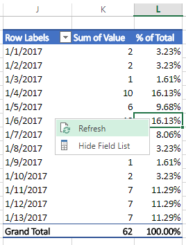
Refreshing PivotTables in Excel Online requires a right-click of the PivotTable > Refresh:

Notice there aren’t the usual plethora of options in the right-click menu, including no PivotTable Options. Hopefully more will appear soon.

Editing/Updating PivotTable Source Data Range

If you formatted your source data in an Excel Table then you don’t need to edit the source range when you add data to the source, as Tables automatically resize and the PivotTable will include this new data upon refresh.

If you need to edit the PivotTable source data range, you can open the file in Desktop Excel and access the full PivotTable functionality there.

Learn PivotTables

PivotTables are a must have skill for any budding intermediate to advanced Excel user. Building reports with PivotTables can be done in a fraction of the time it takes to build the equivalent report using formulas. Plus, PivotTables can’t be broken, unlike formulas.

Take a moment to check out our PivotTable course.

Well, that’s it for this post. I hope you’ll find inserting PivotTables in Excel Online useful. This was one of the most requested features in Excel UserVoice and the Excel team have listened and delivered. If you have an idea for Excel, please take a moment to post it on UserVoice and get your colleagues to vote for it too.

Please Share

If you liked this please click the buttons below to share.