Did you know we can use a nested IF formula to extend the number of logical tests and therefore, possible outcomes? Simply put, this is multiple IF’s nested in the one formula.
Prior to Excel 2007 the limit of IF's you could nest in one formula was 7. Excel 2007 has increased this to an outrageous 64. I say outrageous, because in most cases if you’re using more than a few nested IF’s in one formula, there’s most likely a more efficient way to perform your calculation. So don’t get carried away nesting!
Watch the Video

Download Workbook from the Video
Enter your email address below to download the sample workbook.
IF Formula
In a previous tutorial we looked at the IF function (singular), which is one of the most versatile functions in Excel, but on its own you’re limited to only one of two outcomes. That is, if the answer to the question I am asking is true, do this, if not, do that.
Before we dive in to nested IF’s I want to recap our singular IF statement example to remind us how the logic works:
=IF(The number of units in column D is >5,Then take the Total $k x 10%, but if it’s not > 5 then take the Total $k x 5%)
So, if the answer to the question is true, you get outcome 1, and if answer is false you get outcome 2.
Nested IF Formula
Now let’s take a look at a more complex problem that a nested IF would solve.
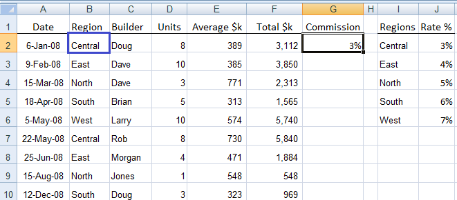
In our spreadsheet below I’d like to enter the commission for each row in column G. The commission rates are different for each region. I’ve listed the different rates in columns I and J so it’s easier to follow.....and later we’ll make the formula more dynamic using this table, but let’s walk before we run.
|
In Excel language our Nested IF statement would read:
= IF(logical_test, value_if_true, IF(logical_test, value_if_true, IF(logical_test, value_if_true, IF(logical_test, value_if_true,.............so on and so on up to 64 iterations)
Let’s translate it into English by applying it to row B of our spreadsheet:
=IF(B2="Central", if so enter 3%, if not see if B2="East", and if so enter 4%, if not see if B2="North", and if so enter 5%, if not see if B2="South", and if so enter 6%, if not see if B2="West", and if so enter 7%, if not enter "Missing")
In Excel it would look like this:
=IF(B2="Central", 3%,IF(B2="East", 4%,IF(B2="North", 5%,IF(B2="South", 6%,IF(B2="West", 7%,"Missing")))))
In the above formula we’re telling Excel to put 3% in the cell if B2=”Central”, if not move on to the next IF statement and so on. In the last IF statement, IF(B2="West",7%,"Missing"), we tell Excel to enter the word 'Missing' in the cell if all previous IF’s are false.
Alternatively we could instruct Excel to enter ‘0%’ or anything else we like in place of ‘Missing’. Or, if we left this argument out altogether Excel would enter the word ‘FALSE’ for us by default.
Let’s make it better
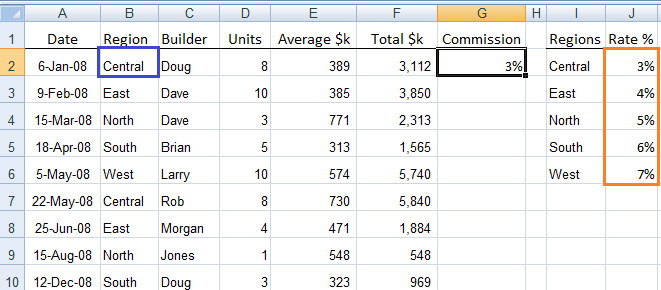
With the formula the way it is we’d have to manually update the percentages for each region if we wanted to alter them. And then copy and paste the revised formula down the column. A better solution would be to link to the table in columns I & J. Then if we updated the percentages in column J, our formula in column G would dynamically update.
For example:
=IF(B2="Central", $J$2,IF(B2="East", $J$3,IF(B2="North", $J$4,IF(B2="South", $J$5,IF(B2="West", $J$6,"Missing")))))
If we wanted to change a rate we’d simply change the rate in column J and it would dynamically update our formula in column G.
|
You could take it one step further and link the IF statement to the region names as well, but I’ll let you play around with that when you download the practice spreadsheet.
I know I said at the beginning that you shouldn’t use more than a few Nested IF’s, and I’ve broken that rule here for the purpose of my example. In reality I would use the VLOOKUP in this scenario as it’s a simpler formula for both the user to interpret later on, and for Excel to compute.
Warning
Too many nested IF's can result in performance issues. In this tutorial you can learn alternatives to nested IFs.

Hi, I have 4 warehouses (columns) listed in Excel. Each associated with a unique sku in each row. If each value in the warehouse shows a qty of 4 or more of a particular sku, I would like it to return a name value. I am having a hard time coming up with a formula for that. Any suggestions?
Hi Sumit,
It’s a bit difficult to visualise how your data is structured. Would you please post your question on our Excel forum where you can upload a sample Excel file and we can help you further.
Thanks,
Mynda
I can see there is a mistake in your statement but not in the formula.
Not sure what you’re referring to, Arun. Can you provide more information?
Hi,I’m having a little trouble sorting a conditional format for a blood pressure chart.the cells concerned are C2 (for the formula) cells D3 & E3.(example) Cell C2 needs to change colour to Orange if D3 is less than 120 or Red if greater than 140 AND/OR IF E3 is less than 60 for Orange and more than 100 for Red
Your help please
Rex
Hi Rex,
Please post your question and sample Excel file on our Excel forum where we can help you. There are too many variables in a conditional format like this to properly answer here in the comments.
Mynda
You might want to add a cross reference to this newer article:
WHEN TO SAY NO TO EXCEL NESTED IFS
https://www.myonlinetraininghub.com/when-to-say-no-to-excel-nested-ifs
Indeed. Thanks for the nudge, Ron. I’ve updated the post.
Cheers,
Mynda
Pff … still learning. Next step using it.
I need a nested IF formula that looks at dates.
If a date in cell B3 minus the date in B4 is equal to or greater than 1 year but less than 3 years, then I want it to return an answer of 40. If B3-B4 is equal to or greater than 3 years but less than 7 years, I want it to return an answer of 80. If B3-B4 is equal to or greater than 7 yrs but less then 15 yrs, I want it to return an answer of 120 and if B3-B4 is equal to or greater than 15 years, I want it to return an answer of 160. I can get the correct answer when using just the two first logical test, but when I try to put it all together, my return answer for every scenario is 160.
Your help would be greatly appreciated
Thank you
Hi Marsha,
The problem with IF nested statements is that the function stops when a criteria is met and returns an answer, regardless of your other criterias.
Try:
=INDEX({0,40,80,120,160},MATCH(A1,{0,1,3,7,15},1))
Catalin
Catalin
Thank you for your time. I guess I don’t know how indexes work. When I put the index formula in the formula bar for that cell I get a result of True when I need a result of 40, 80, 120 or 60
I’m trying to take each employee’s hire date, subtract their anniversary date to get a result of how many hours vacation time they are due – 40 hours for their first and second year anniversary, 80 hours for their 3rd through 6 year anniversary, 120 hours for their 7-14 year anniversary and 160 hours for 15 years and over.
Hi Marsha,
Try this file from our OneDrive folder, you can download the file and test it. It’s the same formula and it returns desired values.
Catalin
very good
Thank you, Kathleen 🙂
Thx for such valuable work out
You’re welcome, Khalid 🙂
what would hinder a subtotal formular from responding on 2007
Hi BJ,
Incorrect syntax probably, but without seeing it I don’t know. You can send your file to me at the help desk and I’ll take a look.
Kind regards,
Mynda.
how i use nested if’s function more than 15 times
Hi Jai,
There are a lot of ways to nest an IF statement.
Here’s my favorite technique:
IF Criteria
True Value
False Value –replace with new IF… IF Criteria
True Value
False Value –replace with another IF and so on
Example:
Data is A1 i.e. 1
Formula is in B1
=IF(A1=1, “ONE”, IF(A1=2, “TWO”, IF(A1=3, “THREE”, IF(A1=4,”FOUR”, IF(A1=5,”FIVE”, IF(A1=6,”SIX”, IF(A1=7,”SEVEN”, IF(A1=8,”EIGHT”, IF(A1=9,”NINE”, IF(A1=10,”TEN”, IF(A1=11,”ELEVEN”, IF(A1=12,”TWELVE”, IF(A1=13,”THIRTEEN”, IF(A1=14,”FOURTEEN”, IF(A1=15,”FIFTEEN”,”BLANK”)))))))))))))))
Please copy and paste this formula in the formula bar while in B1 (and not in the cell) and if Excel asks to check the error just click “yes”.
Now the formula shows 15 IFs nested in this example. If value in A1 is 1 then “ONE” if 2 then “TWO” and so forth and so on.
See IF BASICs
Cheers,
CarloE
in data validation [ list ] unable to use this formula
please help
thanks
Hi jai,
Please send your file with your concerns here: Help Desk.
Cheers,
CarloE
Hi Carlo,
I’m hoping you might be able to construct this formula so it gives me the correct outcome I need in my speadsheet. It is a sharetrading spreadsheet I’m putting together and I’m trying to use nested ifs to make this work.
I have the total value amount purchased in a cell then the next cell across contains the brokerage fees value depending on the amount purchased.
Transaction amount Brokerage fee*
$0 to $5,000 $15.00
$5,001 to $10,000 0.30%
$10,001 to $30,000 0.20%
$30,001 to $50,000 0.16%
$50,001 + 0.12%
Working out your brokerage
Different brokerage rates will apply to each component of
your trade value above $5,000 based on the levels above.
For example, if you placed a $35,000 trade your total
brokerage would be $78.00. This is calculated as follows.
Trade component Brokerage fee Total
First $5,000 $15.00 $15.00
$5,001 to $10,000 0.30% x $5,000 $15.00
$10,001 to $30,000 0.20% x $20,000 $40.00
$30,001 to $35,000 0.16% x $5,000 $8.00
Total brokerage $78.00
Thank you for any solution and really looking forward to the construction of this formula.
Kind regards
Max
Hi Max,
Please check this formula out. Assumption here is that the value is in A1.
Note: I have noticed that when you copy the formula in the cell, it will come out as a text. I prefer you paste it in the formula bar. Just click yes whenever you are prompted by a question that Excel wishes to correct your formula.
Cheers,
CarloE
Hi Carlo
Thank you ever so much, works a treat.
Microsoft Office Excel asked to accept a correction which they deleted the = sign in the first bit (A1<=5000 to (A1<5000
I understand the way you constructed it now, very very clever.
I have only come across this site today and to get solution back so fast is astonishing and very much appreciated. I have already saved the site in my favorites.
Once again Carlo, thanks for your time, effort and goodwill.
Kind Regards,
Max
Hi again Carlo,
To leave the cell empty if A1 has no value I guess I would put a comma & “” after the *0.0012
Such as *0.0012,””)))))
Is this the correct place?
Thanks again Carlo
Cheers … Max
Hi Max,
Just enclose the main IF with another IF .. IF(A1=””,””, Main IF)
like this:
Cheers,
CarloE
Hi Max,
On behalf of Mynda,
You’re welcome.
Cheers,
CarloE
Hi Carlo,
Ahhhhhhhh, very good.
Thanks once again and my thanks also goes out to Mynda.
Just fantastic.
Cheers … Max
Hi Max,
Our pleasure!
CHeers,
CarloE
Great info!
Hi Rick,
Kind words you’ve got right there.
On behalf of Mynda, Thank You!
Cheers,
CarloE
TRYING TO FIGURE OUT IF I CAN USE =IF() STATEMENT IN MY WORKBOOK TO ACHIEVE… WHAT IT IS IM TRYING TO ACHIEVE. LOL. ANYWAY.
SO I HAVE TWO WORKSHEETS IN MY WORKBOOK. ONE TITLED “INC_ASSESSMENT” THE OTHER TITLED, “SHOP_PARTS_TRACKER”.
ON THE “INC_ASSESSMENT” WORKSHEET I HAVE IN CELLS B2:R2 A PLACE TO INPUT SERIAL NUMBERS.
ON THE SAME SHEET CELLS B59:B83 HOUSE A SIMPLE =IF FORMULA TO AUTO-FILL INFORMATION. IN THIS CASE ITS PARTS. =IF(B2,2,0) =IF(B2,4,0) AND SO FORTH…
THIS ALL WORKS GREAT, HOWEVER I NEED MORE FROM THIS EQUATION.
ON THE SAME SHEET IN CELLS B3:R3 I AM USING THIS FUNCTION…
=IF(SHOP_PARTS_TRACKER!H13>0,B2&”R”,0). IT IS LINKED TO THE SECOND WORKSHEET AND ALL IT TRULY DOES IS COPY THE NUMBER FROM THE CELL ABOVE AND PLACE A R NEXT TO IT TO SHOW THAT WE HAVE RECEIVED PARTS FOR THE UNIT.
HERE’S THE NEED I CANT FIGURE OUT HOW TO WORD IN EXCEL SPEAK.
I NEED THE CELLS B59:B83 TO ALSO CHANGE WITH CELL B3, AND WOULD LIKE THEM TO READ “RECEIVED” IF A NUMBER GREATER THEN 0 IS INPUT IN CELL H13, OR RUN THERE STANDARD FUNCTION OR =IF(B2,2,0)
CAN ANYONE HELP ME WITH THIS?
Hi Fran,
I hope I got this right.
Try this formula.
More on IF STATEMENTS.
Cheers.
CarloE
Hi Mynda,
I need to custom the column into 7 digit but the current data i have contains one (1) to seven (7) digit. Can I use this formula to custom the data and translate it into 7 digit?
Sample
Column A Column B
1 0000001
12 0000012
123 0000123
1234 0001234
I want to translate the column A just like the data in column B.
Thank you.
Hi Jezryl,
Use TEXT function.
Cheers.
CarloE
It may be asking too much but I would like to write an IF statement based on time (in one cell) for the following and keep getting an error even when i try to do only the first line. This is what I tried:
=IF(AND(H4300:03:58)”3″,”N”)
=0:3:58,”3″
=0:04:03,”2.5″
=0:3:40,”2.5″
>=0:4:14,<=0:4:24,"2"
=0:3:15,”2″
>=0:4:25,<=0:4:35,"1.5"
=0:3:00,”1.5″
0:4:36,”1″
Hi Susan,
You might want to send your file with some explanation of the algorithm/logic of your formula
via HELP DESK.
In the meantime, try TIME FUNCTION to make your criteria work.
Cheers.
CarloE
Hi
I would *really* appreciate your guidance on my attempted nested equation. Here’s how I’ve it- but I think there must be something wrong as the ‘Or’ bit doesn’t seem to work (B14 is meant to increase by a value of 1).
=IF(AND(A13=A14,B13+B14>=1)*OR(B14>=1),A14+1,A14)
thanks – very helpful site
nb. sorry, reading that back, that was unclear. B14 *is* equal to 1, so the cell the above equation is in is meant to +1… but it doesn’t seem to change its value.
Hi Tom,
I couldn’t quite get what you mean here but I tried to understand this anyway:
your formula should look like this:
here’s the pseudo-formula
IF (A13=A14 AND B13+B14>=1);
OR B14>=1 then
A14 + 1
ELSE(false value of if)
A14
Please you may also send your file through Help Desk for clarification.
See also NESTED IF
Sincerely,
CarloE
I need a nested IF statement to display the season corresponding to a date. For example, if I enter a date (dd/mmm/yy) in a cell, I want another cell to show “Spring”, “Summer”, “Autumn” or “Winter”. I can’t get Excel (ver 2007) to understand what is meant by: =IF(A1=”01 Mar”, “Spring”,”X”)), etc. etc. Can you help please? (Your instructions are very clear & a great help – well done)
Hi James,
Here’s the nested formula that I have created:
=IF(AND(MONTH(A1)>=3,MONTH(A1)<=5), "SPRING", IF(AND(MONTH(A1)>=,MONTH(A1)<=,"SUMMER, IF(AND(MONTH(A1)>=9,MONTH(A1)<=11),"FALL","WINTER"))) So in your case, If you have your date in A1 you can validate it with the formula above To Follow this one here's the pseudo-formula I have diagrammed: 1st IF(Criteria,"TrueValue", 2nd IF(Criteria,"TrueValue", 3rd IF(Criteria,"TrueValue", CatchAllValue) Please note that each IF function is cut-off in its false value until the catch-all value is arrived at. Hence, if we look at the basic syntax IF(Criteria,"True Value", "False Value"), the False Value is replaced with a new IF Function until the Catch-All Value or the False Value for the Main IF Function --which is actually the first-- is arrived at. Click Here for more on IF Functions
Sincerely,
CarloE
=IF(E26=1,($D$5*$B$5),IF(E26=T,($D$5*$C5),0)) Whats wrong with my formula, it brings a “NAME” error
Hello Jackie,
Inside your Outcome 2 = IF(E26=T the letter T should have quotations.
You’ll need the “” sign for Excel to recognize that you are commanding IF Formula to look for TEXT.
So it should be: IF(E26=”T”.
Other than that, I think your formula is perfect.
Just to make sure, have you checked the other cells if you referenced TEXT?
Hope this helps. 🙂
Thanks!
Mike
Thanks for help me The online training Hub
You’re welcome, Ajit 🙂
Thanks, they were usefule.
Thank you, Hamid 🙂
Need tips on nested if statemetns
Hi Michael,
Have you got a specific question on a nested IF statement that I can help you with?
Kind regards,
Mynda.
Hi Mynda, I’m going cross-eyed trying to work out how to do (what seems to me to be) a complex IF formula. I have a table with a range of numbers of games played and a payment range according to the number of games played. Is there a way of saying IF the number in cell A8 falls between (say) 16 and 40 then payment is $40, but if the number in cell A8 falls between (say) 41 and 100 then payment is $100, etc etc – there are five different ranges and the final one is if the number in cell A8 is greater than 150. I’ve tried using >= and <= in the one logical test, and in the final logical test false is not an option as after all that testing the number must be greater than 150 (if you get my drift).
Hi Karen,
You’d be better off using a VLOOKUP formula with a sorted list like this.
Kind regards,
Mynda.
Really help when you don’t remember how to finish whole formula.
Glad to have helped 🙂
Looking forward to some great tips.
Very helpful
Are you able to have two side by side IF’s (not nested) and have them link to one another without bringing up an error?
I mean side by side in the same formula, not in different cells.
Um, no! However, I’m sure there’ll be a solution to whatever it is you’re trying to do. Can you give me an example of your conundrum?
cool, thanks
AC
Thanks for the info