Named Ranges in Excel are an essential tool for simplifying and enhancing the functionality of spreadsheets. They allow you to assign a descriptive name to a cell or range, which you can use in formulas and references instead of cryptic cell addresses like A1 or B2:D10. This makes your formulas easier to read and manage, especially in complex workbooks.
Table of Contents
- Get the practice file
- What Are Named Ranges?
- Benefits of Using Named Ranges
- How to Create Named Ranges
- Named Constants
- Managing Named Ranges
- Using Named Ranges in Formulas
- Tips for Best Practices with Named Ranges
- Advanced Techniques with Named Ranges
- Named Ranges in Tables
- Common Errors with Named Ranges
- Conclusion
Free Practice Workbook and Cheat Sheet

Enter your email address below to download the sample workbook.

What Are Named Ranges?
A Named Range is a custom name assigned to a range of cells, a constant value, or a formula. Instead of typing cell references into your formulas, like
=SUM(A1:A10)you can assign the range a meaningful name, like "Sales" or "ProfitMargin."
So your formula becomes:
=SUM(Sales)which is more intuitive, and it remains consistent even if the cell range changes.
Benefits of Using Named Ranges
- Improved Readability: Names like "TotalExpenses" are much easier to understand than
=SUM(B5:B20).
- Easier Maintenance: Update the range or the value in one place, and Excel automatically updates all formulas using that name.
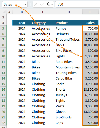
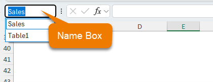
- Faster Navigation: You can jump to Named Ranges quickly by selecting them from the Name Box.
How to Create Named Ranges
There are a few ways you can create named ranges:
1. Manual Creation:
- Select the range of cells you want to name.
- Click on the Name Box (next to the formula bar - see image above).
- Type your desired name (e.g., Sales) and press Enter.
2. Using the Ribbon:
- Select the cells you want to name.
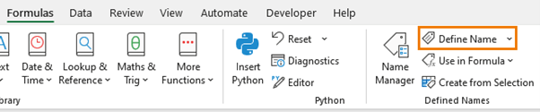
- Go to the Formulas tab.
- Click Define Name, assign a name, and provide optional comments.
3. Create from Selection
If your data is in a table, you can use the table row and column labels to automatically define names:
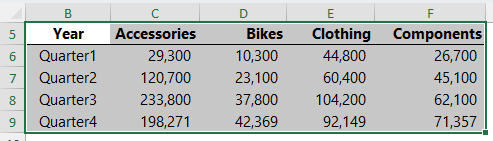
- Select the data in the table including the row and column labels
- Go to the Formulas tab.
- Click on Create from selection
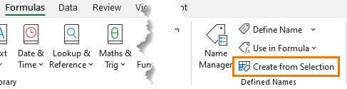
- Check the boxes for the values you want to create names for:
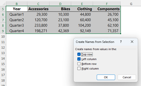
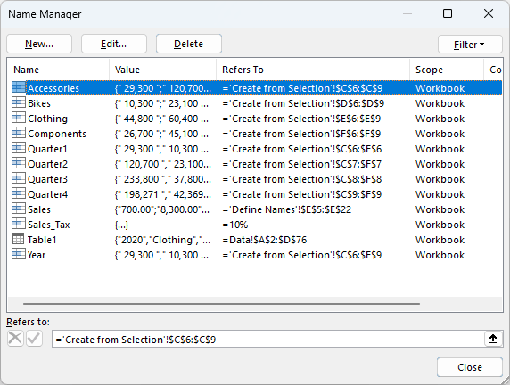
You will now have names automatically defined and available to work with as shown in the Name Manager below (more on the Name Manager coming up):

Named Constants
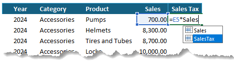
Another clever use of Named Ranges is to define constants. For example, you might frequently use a tax rate or commission percentage across multiple sheets. Instead of typing the value into every formula, you can define a Named Range for that value, like SalesTax = 0.10.
Now, whenever the tax rate changes, simply update the Named Range, and all related formulas update instantly.
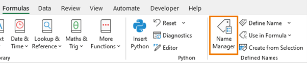
Managing Named Ranges
Once you start using Named Ranges extensively, you'll need a way to manage them. Excel provides the Name Manager, which is located under the Formulas tab.
In the Name Manager, you can:
- Edit existing Named Ranges.
- Delete ranges you no longer need.
- Filter by name or scope (workbook or worksheet).
Tip: You can also use Ctrl + F3 as a shortcut to open the Name Manager.
Using Named Ranges in Formulas
One of the greatest benefits of Named Ranges is their use in formulas. Instead of referencing cells like
=A1+B1you can reference
=Revenue+ExpensesNamed Ranges can be used with all Excel functions, including SUM, XLOOKUP, IF, and others.
Example:
Let's say you've defined a range for your sales figures as Sales. Instead of using
=SUM(E5:E22)you would write:
=SUM(Sales)
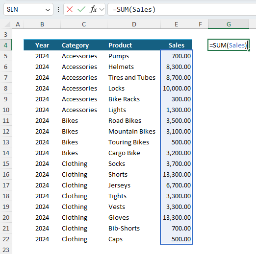
This simplifies your formulas and makes them more readable for anyone reviewing your work.
Tips for Best Practices with Named Ranges
1. Use Descriptive Names: Instead of short names like "A10", use clear, descriptive names like "TotalSales" or "CustomerData" for easier understanding.
2. Avoid Spaces: Names can't include spaces, so use underscores or camelCase (e.g., TotalSales or Total_Sales).
3. Global vs. Local Scope: A Named Range can either have a workbook-wide (global) or worksheet-specific (local) scope. Note: scope cannot be changed once the name is defined.
- If you set the Named Range to have a scope of the whole Workbook you can reference it on any sheet in the Workbook.
- Or if you set it to have a scope of the Worksheet, you can only reference it on the Worksheet you specify when setting up the Name Range.
4. Naming Limitations: Names can't exceed 253 characters and must begin with a letter, underscore, or backslash. Avoid using Excel's reserved names (e.g. "R" or "C").
Advanced Techniques with Named Ranges
While creating a static Named Range is simple, you can take it a step further with more advanced techniques.
Non-contiguous Ranges
You can set non-contiguous Named Ranges by holding down the CTRL key while you highlight the cells you want to name.
Dynamic Named Ranges
Dynamic Named Ranges automatically adjust their size based on the data in the range. This is ideal when your dataset grows or shrinks over time.
For example, if your data is in column A, you can create a dynamic range using the formula:
=OFFSET(Sheet1!$A$1,0,0,COUNTA(Sheet1!$A:$A),1)
This range will expand or contract as the number of rows in column A changes.
Check out our comprehensive post on dynamic named ranges for more.
Named Ranges in Tables
Excel Tables have built-in dynamic ranges called Structured References, so if you add new data to a table, the Structured References will automatically update.
A table structured reference consists of the table name followed by the column name e.g.:
Sales[Budget]
And you can use them in formulas like so:
=SUM(Sales[Budget])
Tables are one of Excel's hidden gems with loads of productivity benefits for using them. Find out more about Excel Tables and their magical properties in our comprehensive Excel Tables tutorial.
Common Errors with Named Ranges
While Named Ranges are a powerful tool, they can cause confusion if not used carefully:
1. Overlapping Ranges: Ensure that your Named Ranges don't overlap unless it's intentional, as this can lead to incorrect calculations.
2. Duplicate Names: If you use the same name across multiple sheets, be mindful of the scope. If you refer to "Sales" but have two ranges with that name on different sheets, Excel may not always use the one you intended.
3. Circular References: Avoid using Named Ranges in formulas that refer back to the same Named Range, as it may cause a circular reference error.
Conclusion
Named Ranges are an incredibly powerful feature in Excel, making your formulas cleaner, easier to read, and more maintainable. Whether you're managing simple lists or complex financial models, Named Ranges help streamline your workflow and reduce errors.
By mastering both basic and advanced techniques, such as dynamic named ranges and Named Constants, you'll elevate your Excel skills and build more efficient spreadsheets.
Start integrating Named Ranges into your spreadsheets today, and experience the difference they make in simplifying your Excel work!


Oustanding Mynda! Best regards from Limón, Costa Rica!
Thanks so much, Jerry!
I am working on impact ratings High, Medium, Low, Nil. How do I average the occurences of this in one column. I assigned values 4-0 to each one but not sure it is correct, although I got numerical values. Could you please help? Thank you.
Hi Sheila, please post your question on our Excel forum where you can also upload a sample file and we can help you further.
I have an excel platform that is used for computing students result, it has a precessing side and an output side. I don’t want the both sides to show at the same time, I want to create an interface such that when you click on Processor, only the processing side of excel sheet will show and when you click on output, only the output will show. How can I achieve this?
Maybe something like hyperlink buttons to navigate to the different parts of your workbook.
Is there any way to change the scope of a named range once created? Let´s say I just created a named range through the name box. By default, the scope is the “Workbook”. If I decide afterwards that I want it to be “worksheet” scoped, how can I modify it?
Thanks
Merry Xmas!
Hi Manuel, no, the only way to change the scope is to delete the name and recreate it.
I am trying to color band a certain area of my worksheet which I’ve defined as a named range. I also have a command button that copies and adds the row before it. Is there anyway to define function that adds color banding as I add rows? I am assuming the VBA code is copying both the formatting and the formulas from the above row. Is there anyway to only have it copy the formulas and the borders without the fill?
Hi Nicole,
You might like to change the code to ‘paste formulas’ which is available in the Paste Special dialog box.
Mynda
Hi,
I’m unable to use the markup function it keeps giving me an error of #NAME?
Hi DG,
Please upload a sample file on our forum so we can see what’s wrong.
Cheers,
Catalin
without a workbook to download, I got lost pretty quickly
Hi Ted,
The workbook download link is towards the top of the post. It’s under the second heading.
Mynda
Thank you! This is exactly what I was needing for my Data Validation lists, as I was out of character space for the items, and we share the workbook, so can not use tables. This worked great, now will not have to update 12 sheets for just adding one new type. Just update one list on a separate worksheet and it is done!
Wonderful! Glad it will help 🙂
Mynda
Thanks for the explanations and tips on uses!
You are the best
Thank you
Excellent! I’ve used Excel for years and never even realized there was a Formulas tab. Wow,can’t wait to subscribe:-)
Glad we could help, Lynne 🙂
Thank you very clear just i have a problem.
I have a formula like sum(first) ,name first = a2:h2
when i copy to another cell down i have the same result because the sum retain the name and don’t change the rows(to 3)
I have no $ at my name and now i have at row 2 sum(first) and at row 3 sum(first) ?
thank you
Hi Walter,
A Defined Name is not aware of the locations where this name is used.
You have to write the formula in a different manner, like:
=SUM(OFFSET(first,0,0)) (or =SUM(OFFSET(first,ROW(A1)-1,0)) for a dynamic formula)
To sum the next row below first, change the offset row to 1:
=SUM(OFFSET(first,1,0)) (the dynamic formula based on ROW function will do that without manual adjustments)
Catalin
VERY HELPFUL INDEED
Thanks, Syed. Glad we could help 🙂
Hi Mynda,
Great site as others have noted.
I`ve used dynamic ranges in the past using the offset functionality, it`s bulky cumbersome and can`t be used in a dropdown list IIRC.. but this new table feature that I`ve just found out about thanks to you does pretty neat stuff indeed…
So the problem is that I want to ignore the header for my data validation dropdown list… is that possible
Thanks,
Thomas
Hi Thomas,
You can use a dynamic range using OFFSET for your data validation source, assuming that’s what you mean by ‘dropdown list’, as opposed to a Combo Box form control.
Another way to build a dynamic named range is using INDEX, as described here.
However, the easiest way is to use an Excel Table as the source for your data validatopm list. There are 3 approaches to this as explained here, and they all ignore the header.
I hope that helps.
Mynda
In older versions of Excel (circa 2003), a named range could be saved in a user’s Personal.xls workbook, which referred to a range in another workbook (i.e., a range not actually in Personal.xls). Once in place, this named range could be referenced by formulas in any other workbook, and as long as the user was working on the same PC/network account with the Personal.xls open/running in the background, the formulas would work. I am now using Excel 2010 and I cannot seem to achieve this same functionality. Personal.xlsb will allow me to save the named range, but my other workbooks cannot “see” or use the name unless I redefine the range, which defeats the point of defining the range in the first place. Any tips?
Hi Chris,
I haven’t tried it but are you prefixing the name with the workbook name e.g.:
=personal.xlsb!your_named_range
Mynda
Yes, the range is defined in my Personal.xlsb workbook with the full network path, file name, worksheet name, and cell range. Here is the actual ‘Refers to:’ string copied straight from Excel:
=’G:\PLANNING\XFILES\PLANNING\ZIP_Codes\[SD_County_zip_code_summary.xlsx]Master_Zip_Listing’!$C$3:$AT$193
Ok, and let’s say the name for this reference string in Personal.xlsb is ‘Master’?
Are you referencing it with:
=Personal.xlsb!Master
And is your Personal.xlsb workbook open?
Mynda
Referencing it as you suggested (Personal.xlsb!Master) works! Thank you so much! However, I am disappointed that I now need to reference it in this fashion – in the older versions of Excel (like 2003), it was not necessary to include the “Personal.xlsb!” portion – simply including the name (Master) in the formula produced the desired result. Thanks again for your help.
Hi Chris,
Glad it’s working now, albeit with a bit more effort required.
Kind regards,
Mynda
There are some excellent tips in here! Thanks.
Thank you!
Great summary book….every one who uses Excel should have this.
Cheers, Jonathan 🙂
YOU ARE DEFINITELY GREAT!
by an Italian in China
Thanks, Denis 🙂
Dear madam,
am unable to make sum(north). could pl help me below details:
MONTH NORTH SOUTH EAST WEST
JAN 100 110 0
FEB 200 11
MAR 100 20
APR 400 88
MAY 400 10
JUN 700 200 110
JUL 800 10 50
AUG 900
SEP 30 400
OCT 1050
NOV 300
DEC 220
Hi Jerald,
Did you name the range that the north data is in? You need to do this first.
Without seeing your file I cannot tell what might be the problem otherwise. You can send us your file via our help desk and we’ll take a look.
Mynda
Mynda, first many thanks for all this great stuff on Excel. I started many moons ago on Lotus 1-2-3. In 123, I could create range name labels, which was useful…. perhaps you’ve already explained it, but can you do this is Excel. That is, if I have a column of Divisions, with the leaders in the column to the right, can I create range names of the leaders of the Divisions.?
Not sure if this will make sense to you…. Thanks for any help you can be.
Cam
Hi Cam,
You can create named ranges quickly from a range of cells. So, if you have divisions in column A and leader names in column B you could highlight the two ranges together then on the Formulas tab of the ribbon in the Defined Names section select ‘Create from Selection’.
This will open the dialog box and you need to check the ‘Left column’ box, then press OK.
You’ll now have named ranges for each division in column A that maps to the leader in column B
I hope that’s what you’re after. If not you could send me an example via the help desk.
Cheers,
Mynda.
Hi, First of all I appreciate that you encourage/advocate sharing knowledge for free (not many in this world do). Your tips are well explained and easy to follow. May the God bless you!
Thank you, Sarath 🙂
Hi Mynda,
Can you help me please , to find a solution for COUNTIFS formula, but with three ore more criteria in same cell: eg
=COUNTIFS(A1:A10,B1:B10,”Jack”,C1:C10,”apple”,D1:D10,”January”,E1:E10,”day&night”),
Mynda i have problem, to count as number, e1:e10 because the excel doesnt know, day&night. I wanna count when I choose day, to be counted, or when i choose night to be counted. ? Thnks a lot
Hi Valon,
Your formula starts with a problem: =COUNTIFS(A1:A10,B1:B10… There is no criteria for the first range.
The syntax of this formula is: COUNTIFS(criteria_range1, criteria1, [criteria_range2, criteria2]…), up to 127 criterias.
For the other problem, as you can add up to 127 criterias, you can use 2 criterias instead of day&night in a single criteria, like E1:E10,”day”,E1:E10,”night”
Your formula should look like:
=COUNTIFS(A1:A10,”which is criteria 1?”,B1:B10,”Jack”,C1:C10,”apple”,D1:D10,”January”,E1:E10,”day”,E1:E10,”night”)
Catalin
Catalin,
Thanks a lot, and I am very appreciate to you.
You helped me a lot,
You’re wellcome 🙂
AFAIK
you can use 2 criterias instead of day&night in a single criteria, like E1:E10,”day”,E1:E10,”night”
doesn’t work in COUNTIFS because it considers the two criteria in an AND relation.
I think you must try with SUMPRODUCT , something like
SUMPRODUCT((A1:A10=”which is criteria 1?”)*(B1:B10=”Jack”)*(C1:C10=”apple”)*(D1:D10=”January”)*(E1:E10=”day”))
+
SUMPRODUCT((A1:A10=,”which is criteria 1?”)*(B1:B10=”Jack”)*(C1:C10=”apple”)*(D1:D10=”January”)*(E1:E10=”night”))
HTH
You’re right Carlos,
thanks for spotting that error.
Your sumproduct version will work fine, but the simplest approach is to write all variables in a single formula, instead of writing again the entire formula for the second variable, like:
=SUM(COUNTIFS(A1:A10,”John”,B1:B10,”Jack”,C1:C10,”apple”,D1:D10,”January”,E1:E10,{“day”,”night”}))
Sumproduct will accept too the list of constants:
=SUMPRODUCT((A1:A10=”John”)*(B1:B10=”Jack”)*(C1:C10=”apple”)*(D1:D10=”January”)*(E1:E10={“day”,”night”}))
Cheers,
Catalin
hi mynda
your Absolute! thanks so match
🙂 You’re welcome, Mano.
hello mam can u pls explain me how to use name manager with the basic i m article in chartered accountant office i want to use it in my office.
Hi Nisha,
This is all I’ve got on the Name Manager in our free training. If you’d like to sign up for our Premium training it is covered in more depth.
Kind regards,
Mynda.
It was suggested elsewhere that I use a range in a formula. I never did it before. I used Mr. Google and found this explanation. WOW! Talk about easy and clear.
I’ve been using MS help inside Excel and it’s close to worthless.
This blog is so easy, logical and complete (as I was reading, questions popped into my head and you answered them about 2 seconds later) I’m going to incorporate ranges into my spreadsheets from now on.
I’ve bookmarked your site and cannot thank you enough!
Mr. Biker,
You’re welcome,
On behalf of Mynda.
Cheers,
CarloE
Is there a way to use the name manager to populate a radio box or some sort of list box in VBA?
So I have X defined ranges in my worksheet. I run a macro that pops up a box that allows me to select the range I want to use and then closes the box.
Hi Matt,
As much as we would like to help you,
VBA is outside the scope we are supporting right now.
The good news is that we are currently developing VBA
programs for Office Apps.
Cheers.
Carlo
Hi,
I would like to know how to rename a named range or extend the range by few more cells when I add new values to the range
Eg; Say I have a list of courses
Course1
Course2
Course3
I would have saved these values as a named range- Courses. How do I add more values to this list and still be able to add it under the same named range?
Please help!
Hi Madhura,
Judging from the way you presented your problem, I bet you are already familiar
with named ranges.
I know you know this already, Go to Formulas ribbon, Click Name Manager, Click New.
Name this as ‘Mylist’
Now here’s the new part, in the refers to box, paste this formula:
Now add a Data Validatation. In the source box, type:
Assumptions:
Sheet1 is the name of your sheet. and your list is in B2:B1000.
So start with your three items and try to add some.
The rest of the story is here:
Everything you need to know is all in this link: DYNAMIC NAMED RANGES
Cheers.
CarloE
That works awesome!
Thanks CarloE
Cheers!
Hi Madhura,
You’re much welcome. It’s Mynda’s blog post and I just learned it from her.
Thank Mynda!
Cheers.
CarloE
I would appreciate any help you can provide. I’m using a SUMPRODUCT formula which is summing multiple values that are present within a Named Range. This works great until the Named Range values are not contiguous at which point I get the #VALUE! error. I’m not sure why this is happening. The formula is the same. Should the fact that the Named Range is non-contiguous matter? Thanks.
Hi Tim,
I would appreciate it more if you can send your file through Help Desk with some sample data and your formula you’re trying to work out.
Anyway…
I just want to clarify if what you mean is that the Named Range is composed of non-contiguous ranges or if you mean that the Named Range is contiguous but the values in it are not contiguous.
Anyway, if you mean the former, I would say Excel really does return an error for that (I would suggest for a workaround if you can send me your file). If you mean the latter, As long as the Named Ranges referenced are of the same dimension I don’t think there will be an error.
Sincerely,
CarloE
Thank you for the excellent tutorial.
Nathan
Cheers, Nathan 🙂
Hi Mynda,
I have an excel sheet which I am trying to load on a sharepoint page using excel web parts.
My excel sheet has an option button, and also certain fields that are coloured conditionally. I try to create a named range so that I could load the sheet on sharepoint. But I find that the option button and other controls are not included in the named range. Is there any way in which I can ensure that my excel controls are included in the excel named ranges? Also any idea why the colours in the coloured fields are not appearing?
Hi Gans92,
I’m sorry, I’m not familiar with Sharepoint and it’s limitations.
Kind regards,
Mynda.
Dear Sir,
The column is extremely helpful. ITs helped me to understand the Excel with named range which I am using in SpreadsheerGear. IF you can help me to apply the alternate rowstyle to the name range would really very helpful.
Thanks in advance!
Mohini
Hi Mohini,
I’m glad we could help 🙂
I’m sorry, I don’t know what you mean by ‘apply the alternate row style to the name range’.
Kind regards,
Mynda.
Hello Mynda,
Thank you so much for the quick reply.
Here is my problem : Actually I am using Speadsheet gear for Exporting the reports. In this I am preparing the Names (range of the cells). And these names I am referring with their names in the code to populate the data. I am able to populate the data in the names as well as able to apply the formats. But I need to apply the alternate rowstyles for data rows where alternate rows will be colored in gray. I can do this in excel to the table or set of the cells by using conditional formatting but I need to apply the same to the name which I am creating in the excel template. Please help!
Your help will be really appreciated!!
Thanks in Advance !
Mohini
Hi Mohini,
I don’t think you can…every time you enter the named range in the ‘Applies to’ field Excel converts that range to cell references again.
There is some discussion about it on a Microsoft forum here. There is also a VBA alternate solution.
I’m sorry I can’t be of more help.
Kind regards,
Mynda.
Hello,
About name range, can you help me with this:
I defined a name range (Products) with 2 columns and 40 rows (=Sheet2!$B$2:$C$41). Cells are all strings. I use this definition as a source for a combobox. My problem is that in combobox I see only first column of defined name range (column B from 2 to 41). It is possible to see all range in combobox selection ?
Thanks
Hi Ovi,
I don’t think so! I suggest you create a helper column (let’s say column D) that joins columns B & C together and refer your combo box to the concatenated values in column D.
Kind regards,
Mynda.
Hi Mynda,
Thanks for your quick answer. That’s was my thinking too. But, my first effort was to use sheets as they are… Almost because of end users, you now… I think that I can use a formula for the new column, something about D=B+C, so when B or C changes, also D changes. Any other suggestions ?
All the best,
Ovi
Hi Ovi,
Yes you can concatenate the text in columns B & C like this:
=B1&C1
For more on using the ampersand symbol to concatenate.
Kind regards,
Mynda.
P.S. Oh, yes…I know what you mean about end users 😉
How can I print individual rows 1 row at a time, 1 row per printed page
without having to call out each row to print one at a time manually. I do this function every date up to 50 rows of data and it is time consuming. I would like to just state a range and walk away while it is being printed.
HELP!
Hi Eric,
I’d set my margins so small that only one row fits on each page. I hope that helps.
Kind regards,
Mynda.
Hi Eric / Mynda
I’ve had this issue before, the easiest way I have found is to setup page breaks, for the number of rows you want printed, then save the sheet after use, save as page breaks 5 rows, or something like that, the next time you need this, special paste the data (as values), then excel will remember your setting
Hope it help
Hi Mynda
Excellent site, thank you for you guides, very helpful indeed
Cheers, Adam. Thanks for sharing your idea.
Mynda.
Hi, I tried many things by seeing your website i’m working in a school we use to maintain a data base of the student in excel sheet, it consist of assessment marks of all subjects and converting to grade. when i’m converting it to grade i found i cannot able to convert absentees which have mentioned using “AB” this has to written in the formula. I convert marks in to grade using this formula =IF(E8>=45,”P”,”F”) in the same formula i have to include “AB” if they are absent,.
FOR YOUR CLEAR UNDERSTANDING: I have to check whether they are present or absent, if they are present i have to check whether they are above 45 if satisfies then it has to convert it into “P” else “F”.
Please help me in this so that you
Hi,
You can use a nested IF statement for this.
For example, where A1 contains whether they’re present or absent, and B1 contains their marks:
=IF(A1=”Present”,IF(B1<45,"F","P"))
Kind Regards,
Phil.
thumbs up!!! that’s exactly what I need, very detailed and straightfoward!Really appreciate!
You’re welcome, Karen 🙂
I am trying to improve my Microsoft proficiency and this tutorials are very helpful. Thanks so much for making them available. I will pass them on.
really good to learn
I have two sheets (namely Site and Sumary)
Site
Name SITE Salary budgeted month 30-04-12 31-05-12 30-06-12
A ABC 1000 30-06-2012 1000 1000 1000
B BCA 1100 31-05-2012 1100 1100
C ABC 1200 30-04-2012 1200
D ABC 1300 30-06-2012 1300 1300 1300
In summary sheet, i would like count the number of persons by month with by Site.
I tried countif funtion but doesnot give result. which function i have to use here.
Kinldy help me
Hi Kurian,
I apologise for the late response to your question. We were abroad at the time and unfortunately your question was missed.
I presume you want to count the number of persons based on the data in the ‘budgeted month’ column. If so you could use a formula like this:
=COUNTIFS($B$2:$B$5,”ABC”,$D$2:$D$5,E$1)
Where column B contained ‘Site’ and column D contained ‘budgeted month’ and cell E1 contained ’30/04/2012′. You could then copy this across to columns F and G.
I hope that helps. If not please let me know.
Kind regards,
Mynda.
I would like to learn more in Countif function (in two sheets)
Best Regards
Kurian
First – Great article
I would like to add the following notes:
Long range names can also cause issues as a lot of people don’t know that you can re-size the name box (in Excel 2007 & 2010) so you can read them.
In earlier versions of Excel (which many companies still use) it was not possible to manually resize this box and you needed to use a VBA procedure to auto resize it – which also may not be practical given many companies security restrictions on running macros.
I would also suggest that constants which are often one or more letters can be identified using a descriptor such as const_ for constant, or calc_ for a calculation etc. which allows users to still use terms they are familiar without having to invent new names for something.
Thanks.
Thanks, Dave. Great tips. I didn’t know you could re-size the name box either!
Kind regards,
Mynda.
I created an Excel chart using macros written in Excel 2003. A function of this macro is the create Chart01, copy it to Chart02 then update the data point references in Chart02. However, when the code initializes the copy of Chart01 I receive several “Name Conflicts” messages. I quickly click through the “Use in destination sheet” messages, and everything turns out okay. My question is: What is the cause of this, and how do I correct it? I’ve been using this code for several years, and never had a problem in 2003. HELP!
Hi Thomas,
Excel 2007/2010 doesn’t like the word ‘chart’ to be used in a named range used with charts. You will need to rename your named ranges that containt the word ‘chart’.
Go to the Formulas tab > Name Manager and edit them.
Also because Excel 2007/10 has so many more rows and columns you need to be careful not to abbreviate your named range so that it is the same as a cell reference. e.g. CH1
I hope that helps.
Kind regards,
Mynda.
Is there any benefit (or hinderance) to having a global named range that is listed in the Name Manager multiple times, but with different scopes?
In other words, I have a Data tab as my data source. I then have a Tab1 that references the DataSet range on the Data tab. When I copy Tab1 and make a Tab2 (Tab3, Tab4, etc.), each time I create the new tab it creates a new DataSet range in the Name Manager, but with a different scope. So I end up with something like this:
DataSet Refers to: Data Scope=Workbook
DataSet Refers to: Data Scope=Tab1
DataSet Refers to: Data Scope=Tab2
DataSet Refers to: Data Scope=Tab3
etc.
Does that effect speed/performance at all? Should I delete all the individual names and just have one that says Scope=Workbook? Or does having each one make calculation faster? Or doesn’t it matter either way
Thank you
Hi Jeff,
Great question.
Having multiple named ranges that are the same but with different scopes doesn’t cause performance issues. The named ranges on their own don’t do any calculations (and therefore don’t require any memory) it’s only when you use them in formulas, and even then it depends on what formulas you use them in plus the size of the data range as to whether they may cause performance issues. So having multiple named ranges the same as opposed to different names makes no difference to Excel’s performance.
Just to be clear on how the named ranges work: Say the named range ‘DataSet’ on Tab1 refers to the cells on Tab1 (say A1:A10), and it has a scope of ‘Workbook’, this means you can use the named range in a formula anywhere in the workbook. (It doesn’t refer to the same cell range on all sheets in the workbook.)
And, the named range ‘DataSet’ on Tab2 refers to the cells on Tab2 (say A1:A10), but you can only use that named range in a formula on Tab2 because the scope for that named range is ‘Tab2’.
You cannot have a named range that refers to cell ranges on multiple tabs/sheets.
So, what may be an issue is the confusion caused from having multiple named ranges with the same name. You would be better off having a separate named range for each tab, say Tab1_DataSet, Tab2_DataSet etc. and each having a scope of the workbook.
Another reason for having different named ranges is if you ever wanted to do a summary page that summed the named ranges for each tab you would need to have a unique named range for each tab with the scope ‘workbook’ for each. e.g. =SUM(Tab1_DataSet,Tab2_DataSet,Tab3_DataSet,Tab4_DataSet).
I hope that makes sense.
Kind regards,
Mynda.
I found this very interesting. I am a trainer helping teachers understanding Excel and its components.
Is there something for Excel 2010 – Pivot Tables?
Hi Peter,
Thanks for your feedback.
PivotTables in Excel 2007 and 2010 are almost identical. 2010 offers some additional functionality like slicers and larger data set capabilities, but the way you create a PivotTable and set options etc. is unchanged from 2007.
You can read my PivotTable tutorial here.
Kind regards,
Mynda.
Hi Teacher,
I want to use IF, COUNTIF,COUNTIFS,SUMIF,SUMIFS functions in a single cell. Please guide me with some examples.
Hi Ranju,
Why would you want to do that!? Sure I can come up with a scenario but it may not apply to your needs. What would help me serve you better is if you were to give me an example of what you’re trying to achieve and I can offer you a solution, that may or may not need to use all those functions in a single cell.
I look forward to hearing back.
Kind regards,
Mynda.
HI, I am learning all about Name Manager and your blog was very insightful. I have a question which I hope you might be able to help me. I have a massive list of names that are assigned to a specific category…Doe, John = Sunshine, Doe, Mary = Sunshine for example. This works great when I add them in Name manager and test it in my formula. My question is when it is not Doe, John or Doe, Mary I want to label this differently = Rain for example. So, without having to type all the names which are thousands is there a way I can describe that in one cellin Name Manager and it understands if not doe, john or doe, mary then = rain. Help!
@Palliana
Thank you for your question. I’m having a little difficulty understanding exactly what you mean but I’ll have a guess.
I think you’re saying you’ve got a list of names e.g. Doe, Mary and Doe, John that belong to a named range called Sunshine and other names that belong to a different named range called Rain.
But not all of the names are in Excel, and therefore you’d need to type them in so you can tell Excel what named range they are in….but you want a quicker option.
If this is the case it may be possible to use a formula (like an IF statement) to perform whatever calculation you want without the need for a named range in the first instance, but without knowing what the end result is I can’t advise you on what this formula should be.
However, if you want/need to use named ranges unfortunately you will have to import, or type the names into Excel and give the categories a named range. There’s no ‘formula’ type of logic in the Name Manager that will allow you to tell it that all ‘these’ names are in the Sunshine category and any ‘others’ are in the Rain category.
If your names (Doe, John etc) are in another system are you able to import them into Excel?
I hope this helps. Please let me know if I’ve misunderstood your question.
I know this is really boring and you are skipping to the next comment, but I just wanted to throw you a big thanks – you cleared up some things for me!