Excel MROUND function is perfect for rounding numbers to the nearest multiple.
For example, last week Brenda said she was making a timesheet and wanted to round the start and finish times to the nearest 15 minutes while allowing for a 7 minute grace period. The table below has some examples:
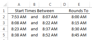
Rounding these times to the nearest 15 minutes is easy with the MROUND function, like so:
=MROUND(A2,"0:15")
Take note of the double quotes around the 0:15 in the formula above. More on that in a moment.
Warning, boring stuff ahead.
Excel MROUND Function Syntax
MROUND is available in Excel 2007 onwards.
The syntax for the MROUND function is:
MROUND(number, multiple)
Where number is the cell or value you want to round, and multiple is the multiple you want to round your number to.
MROUND rounds up away from zero if the remainder left after dividing your number by the multiple is greater than or equal to half the value of multiple. What!?
Sorry, but I warned you it was boring 😉 Let's look at some examples as it will make more sense....hopefully.
Rounding Numbers with MROUND
When working with time the multiple is entered in a time format "h:mm" surrounded by double quotes, as you can see in the first example above, which was:
=MROUND(A2,"0:15")
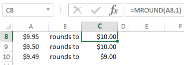
However, when using MROUND to round regular numbers you simply enter the multiple without the double quotes. For example; let’s say we have some prices that we want to round to the nearest dollar as shown below:
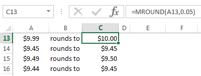
Or maybe you're pricing products and want to round to the nearest 5 cents:
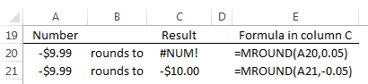
Rounding negative values requires you to use the same sign in the ‘multiple’ argument otherwise you get a #NUM! error:
More Rounding
MROUND will round up or down to the nearest multiple, but if you want to fix the direction of rounding you can use:
Or

First of all, your tips are never boring, Mynda!
Secondly, Mround is available in earlier versions of Excel. It just did not show up in the function list. This is from Alan Wyatt 01/08/16, “This function is provided as part of the Analysis ToolPak; it is not inherent to Excel. To use it, install the Analysis ToolPak (which many people do when Excel is first installed), and then choose Add-Ins from the Tools menu to make sure the Analysis ToolPak is selected.”
Thanks for the Pivot table course. Always fun to learn new tips and tricks.
Good to know….although I hope no one is still using Excel 2003…or earlier 🙂
Another point of attention with regard to MROUND is the use in combination with implicit intersection or in array formulas.
Suppose you have defined names Amount for numbers in A2:A5, and Multiple for multiples in B2:B5.
=MROUND(Amount,Multiple) in C2 will return a VALUE#! error as MROUND doesn;t recognise implicit intersection.
However, if you use Amount and Multiple in combination with a formula or calculation, it will work for you, e.g.
=MROUND(–Amount,–Multiple) in C2 will return the correct result.
The same phenomenon and remedy apply to the use of MROUND in array formulas.
Interesting, Marcel. Thanks for sharing.