Extract Text from a Cell using MID Formulas

Last week we looked at how to use Excel’s Text to Columns tool to extract the domain name from a URL.

Today we’re going to look at how we can achieve the same result using a formula like this one displayed in the formula bar below:

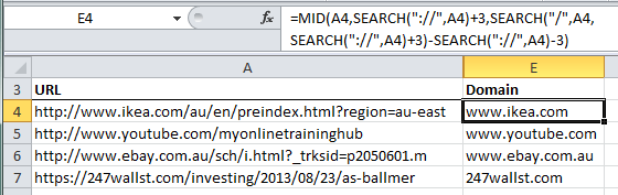
Don’t be put off by its length. First we’ll step through how this formula works and at the end I’ll show you a system for building formulas like this in a few easy steps.

Note; we’ll use the Ikea URL in cell A4 throughout this example.

Let’s start with the functions used in the formula above:

SEARCH or FIND

SEARCH and FIND are almost identical; the only difference being that FIND is case sensitive, whereas SEARCH is not. I have used SEARCH but if you need a case sensitive match then use FIND.

FIND returns the starting position of one text string within another text string and IS case sensitive. The syntax is:

FIND(find_text, within_text, [start_num])

SEARCH returns the starting position of one text string within another text string and is NOT case sensitive. The syntax is:

SEARCH(find_text, within_text, [start_num])

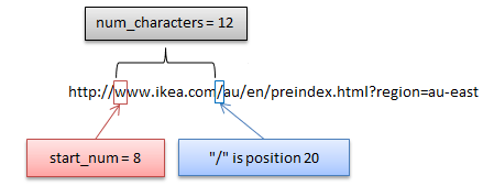
For example the first ‘w’ in the Ikea URL is in position number 8:

http://www.ikea.com/au/en/preindex.html?region=au-east

In this example I've used the SEARCH function to return the arguments for the MID function.

MID

MID returns the characters from the middle of a text string, given a starting position and length. The syntax is:

MID(text, start_num, num_characters)

The start_num we want is 8 i.e. the position of the first ‘w’ in the URL, and the num_characters for the domain is 12 i.e. ‘www.ikea.com’ is 12 characters long.

So we now know that our MID formula should be:

=MID(A4,8,12)

However since each domain is a different length we want to automate the tasks of finding the start_num and num_characters.

To do this we’ll use the SEARCH function to locate a character or characters that are on either side of the domain name and are common to each URL, (known as delimiters).

Identifying Delimiters

First let’s choose what delimiters are common to each URL.

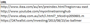
We can see that every URL has the text string :// before the domain name.

The location of this text string in the Ikea URL is 5 i.e. the colon in :// is the 5^th character in the URL. We then add 3 to this (:// is 3 characters) to give the position of the first ‘w’ which is 8. This will be our start_num argument for the MID function.

We can also see that at the end of each domain is another forward slash /. Locating this will help us calculate the num_characters argument for the MID function. In the Ikea URL the first single / is in position 20.

But we don’t want to return 20 characters as this will be too many, so we need to subtract the 8 i.e. the number of characters up to the first ‘w’, from 20 to give us the domain length of 12.

Using SEARCH to Locate Characters

Remember the syntax for the SEARCH function is:

SEARCH(find_text, within_text, [start_num])

Note: start_num is optional for the SEARCH function. It will start at the beginning if omitted.

Here is the formula for the Ikea URL in cell A4, colour coded so we can follow how it works:

=MID(A4,SEARCH("://",A4)+3,SEARCH("/",A4,SEARCH("://",A4)+3)-SEARCH("://",A4)-3)

We'll look at the first SEARCH formula which gives us the MID start_num argument (in this formula we aren’t using the SEARCH function's ‘start_num’ argument):

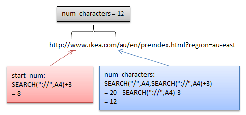
SEARCH("://",A4)+3 

In English it reads; search cell A4 and tell me the start number for text string :// then add 3 (remember, we add 3 on the end because :// is 3 characters long and we want to return the text starting after the ://) which is:

=8

The num_characters, or length of the characters we want returned is determined by the location of the first forward slash “/” after the domain, minus the number of characters up to the end of ://.

Again we can use the SEARCH function to find the “/” (note: in this formula we are using the SEARCH Function's ‘start_num’ argument to tell the it to start searching after the ://):

SEARCH("/",A4,SEARCH("://",A4)+3)-SEARCH("://",A4)-3

=20-SEARCH("://",A4)-3

=20-8

=12

In English: search for “/”, in cell A4, start your search after the “://” characters +3, minus the preceding number of characters up to the end of :// to get the length of the domain.

This formula will work for each URL in the list, including the URL that starts with ‘https’ as some do.

Tip: if some of your URL’s simply start with www and don’t have the http:// at the front you can use this formula:

=IF(ISNUMBER(SEARCH("://",A4)),MID(A4,SEARCH("://",A4)+3,SEARCH("/",A4,SEARCH("://",A4)+3)-SEARCH("://",A4)-3),LEFT(A4,SEARCH("/",A4)-1))

The above formula checks if the :// is present in the URL and if it is is uses the original formula we looked at, however if it isn’t it returns the characters on the LEFT up to the / -1, assuming the URL is in this format:

www.ikea.com/au/en/preindex.html?region=au-east

System for Building MID Formulas

One of the challenges with building complex MID formulas is getting all the nesting right. Trust me, once you start to nest more than two SEARCH functions you lose track of where you’re up to and you might get that head spinning feeling.

This is why I like to use helper columns to locate the characters using one formula at a time. Once I’ve got all the arguments for my MID function using individual formulas I can nest them into one big formula and get rid of my helper columns.

Here is an example where I want to extract text from the middle of the string in column A in the format displayed in column F (note how all strings in column A are not the same length):

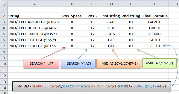
You can see from the image above that I have used 4 helper columns (B to E) before coming to my Final Formula in column F. They are:

Column B: The SEARCH function locates the position of the first space before the text I want to extract.

Column C: The SEARCH function locates the position of the hyphen that I need to exclude from my new text string.

Column D: Uses the result in columns B and C to extract the alpha component of my new text string.

Column E: Uses the result in column C to extract the numeric component of my text string.

Interim Formula

Before building my final formula I first write an Interim Formula in column F that references the results from the SEARCH formulas in columns B and C:

=MID(A7,B7+1,C7-B7-1)&MID(A7,C7+1,2)

I check it’s returning the correct result and then replace the cell references to columns B and C with the actual formulas in those helper columns like so:

=MID(A7,SEARCH(" ",A7)+1,SEARCH("-",A7)-SEARCH(" ",A7)-1)&MID(A7,SEARCH("-",A7)+1,2)

Now I can delete the helper columns and I’m done.

Key Steps

To summarise I take the following steps:

1. Identify the delimiters I can use in my SEARCH or FIND formulas to locate the positions in the text string that are common to all of the strings in column A. In this example it was the first space and the hyphen.
2. Create helper columns to house my SEARCH or FIND formulas that locate the delimiters I need to use.
3. Build an Interim Formula in column F that references the helper columns. Technically the formulas in columns D and E are interim formulas too.
4. Edit the Interim Formula in column F and replace the references to the helper columns with the actual formulas in those helper cells to get your Final Formula.
5. Delete the helper columns.

Don’t forget you could also use Text to Columns to achieve the same results much faster than writing a complex nested MID formula.