In this tutorial, we'll dive into the powerful Excel INDEX and MATCH functions, which are essential for manipulating and analyzing large sets of data.
We'll start by exploring what these functions do and how they retrieve specific information from a table, and then we'll write INDEX and MATCH formulas together as an alternative to the VLOOKUP formula.
We'll also cover some practical use cases for INDEX and MATCH formulas.
Note: if you have Excel 2021 or later, or Microsoft 365 you should use the XLOOKUP function as this is easier and potentially more efficient.
Watch the INDEX and MATCH Video

Download the Excel File
Enter your email address below to download the sample workbook.

Download the workbook. Note: This is a .xlsx file. Please ensure your browser doesn't change the file extension on download.
How the INDEX function works:
The INDEX function returns the value at the intersection of a column and a row.
The syntax for the INDEX function is:
=INDEX(reference, row_num,[column_num], [area_num])
In English:
=INDEX( the range of your table, the row number of the table that your data is in, the column number of the table that your data is in, and if your reference specifies two or more ranges (areas) then specify which area*)
*Typically only one area is specified so the area_num argument can be omitted. The examples below don't require area_num.
INDEX will return the value that is in the cell at the intersection of the row and column you specify.
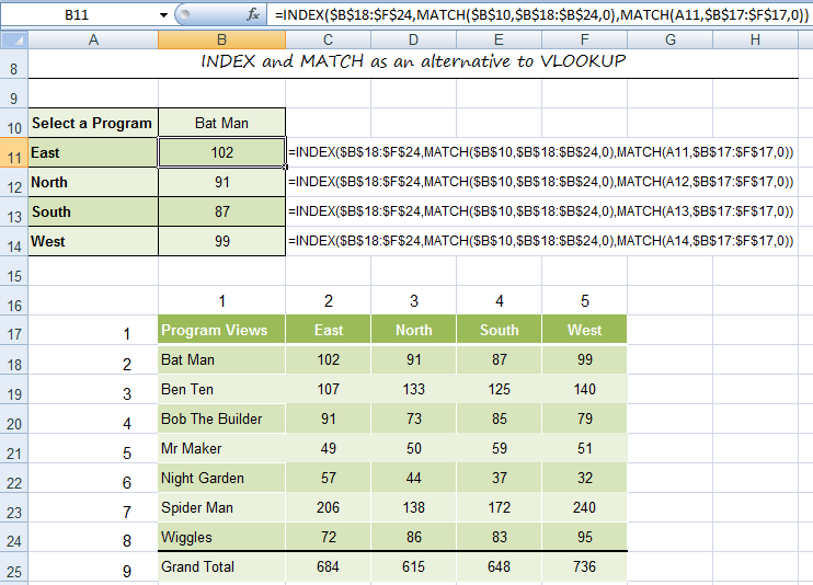
For example, looking at the table below in the range B17:F24 we can use INDEX to return the number of program views for Bat Man in the North region with a formula as follows:
=INDEX(B17:F24,2,3)
The result returned is 91.

On its own the INDEX function is pretty inflexible because you have to hard key the row and column number, and that’s why it works better with the MATCH function.
Note: You may have noticed that the INDEX function works in a similar way to the OFFSET function for creating dynamic arrays, in fact you can often interchange them and achieve the same results.
How the MATCH function works:
The MATCH function finds the position of a value in a list. The list can either be in a row or a column.
The syntax for the MATCH function is:
=MATCH(lookup_value, lookup_array, [match_type])
Now I don't want to go all syntaxy (real word 🙂 ) on you, but I'd like to point out some important features of the [match_type] argument:
- The match_type argument specifies how Excel matches the lookup_value with values in lookup_array. You can choose from -1, 0 or 1 (1 is the default)
- [match_type] is an optional argument, hence the square brackets. If you leave it out Excel will use the default of 1, which means it will find the largest value that is <= to the lookup_value. The values in the lookup_array must be in ascending order when using 1 or omitting this argument..
- 0 will find the first value that is exactly equal to the lookup_value. The values in the lookup_array can be in any order.
- -1 finds the smallest value that is >= to the lookup_value. The values in the lookup_array must be in descending order, for example: TRUE, FALSE, Z-A, ...2, 1, 0, -1, -2, ..., and so on.
Ok, that's enough of the syntax.
In English and using the previous example:
=MATCH(find what row Bat Man is on, in the column range B17:B24, match it exactly (for this we'll use 0 as our argument))
The result is row 2.
We can also use MATCH to find the column number like this:
=MATCH(find what column North is in, in the row range B17:F17, match it exactly (again we'll use 0 as our argument))
The result is column 3.
So in summary, the INDEX function returns the value in the cell you specify, and the MATCH function tells you the column or row number for the value you are looking up.
INDEX MATCH Together:
The INDEX and MATCH functions are a popular alternative to the VLOOKUP. Even though I still prefer VLOOKUP as it’s more straight forward to use, there are certain things the INDEX + MATCH functions can do that VLOOKUP can’t. More on that later.
Using the above example data we’ll use the INDEX and MATCH functions to find the program views for Bat Man in the East region.
=INDEX( the range of your table, replace this with a MATCH function to find the row number for Bat Man, replace this with a MATCH function to find the column number for East)
The formula will read like this:
=INDEX( return the value in the table range B17:F24 in the cell that is at the intersection of, MATCH( the row Bat Man is on) and, MATCH(the column East is in)
The formula looks like this:
=INDEX($B$18:$F$24,MATCH("Bat Man",$B$18:$B$24,0), MATCH(“East”,$B$17:$F$17,0))
So why would you put yourself through all that rigmarole when VLOOKUP can do the same job.
Reasons to use INDEX and MATCH rather than VLOOKUP
1) VLOOKUP can’t go left
Taking the table below, let’s say you wanted to find out what program was on the Krafty Kids channel.

VLOOKUP can’t do this because you’d be asking it to find Krafty Kids and then return the value in column B to the left, and VLOOKUP can only look to the right.
In comes INDEX and MATCH with a formula like this:
=INDEX($B$33:$B$40,MATCH("Krafty Kids",$C$33:$C$40,0))
And you get the answer; ‘Mr Maker’.
Notice only the Programs column (B) was referenced in INDEX's array argument? This means we can omit INDEX's column number argument as there's only one column in the INDEX array.
2) Two way lookup
The table below has a drop down list in B1 that enables me to choose the Sales Person from the table, and a drop down list in A2 for the region. In B2 I’ve got an INDEX + MATCH formula that returns the sales that match my two criteria.
=INDEX(A4:J10,MATCH(A2,A4:A10,0),MATCH(B1,A4:J4,0))

=VLOOKUP(A2,$A$4:$J$10,MATCH(B1,A4:J4,0),FALSE)
Ways to improve these formulas:
1) Use named ranges instead of $C$33:$C$40 etc. to make formulas more intuitive and quicker to create.
2) An alternative to using a named range is to convert the data to an Excel Table whereby Excel automatically gives the table a named range.
3) If there is nothing else in the columns other than your table you could use column references like this C:C which will search the whole column.

How that formula convert to excel 365? this formula
=INDEX(B2:E5;MATCH(A8;A2:A5;0);MATCH(A9;B1:E1;0))
Rizky,
INDEX & MATCH formulas don’t need converting for Microsoft Excel 365, they already work as is. If you’re having trouble with this formula, please post your question on our Excel forum where you can also upload a sample file and we can help you further.
Mynda
HI
I HAVE 2 SHEETS
FIRST SHEET CONTAIN DATA WITH NAME COST PRICE
2 ND SHEET CONTAIN ANOTHER DATA
MY COST PRICE SHEET CONTAIN DATE AS BELOW
ROW 4 DATE
ROW 5 RATE
COLUMN A PRODUCT NAME
COLUMNS B,C,D,E, ETC COST
NEED TO FIND RATE , AT SPECIFIC PRODUCT NAME AND SPECIFIC DATE
AT THE 2ND SHEET G4=DATE C15=PRODUCT NAME
=INDEX(‘cost price’!D5:Q5,MATCH(G4,’cost price’!D4:Q4,1),MATCH(C15,’cost price’!C7:C71,0))
THE RESULT FOR THIS FORMULA IS COLUMN 9 FOR PRODUCT AND COLUMN 9 FOR DATE , BUT THE RESULT OF INDEX:RATE #REF!,
Hi Ali,
It’s a bit hard to follow. Please post your question on our Excel forum where you can also upload a sample file and we can help you further.
Mynda
Hi I need help with this..
A data of 1 Manger in column A to Column A with 4 Team Leads and each team lead has 4 reps.
I would like all reps of Team Lead 4 to be in column D using array index match formula. How should I proceed?
Hi Jaygar,
Please post your question on our Excel forum where you can also upload a sample file and we can help you further as it’s difficult to picture what you’re referring to.
Thanks,
Mynda
Hi !! My INDEX and MATCH formula is working, Value is picked up….But the cell color is not picked up…..Can you please help me out ?
I’m not sure what you mean by ‘the cell colour is not picked up’? Please post your question and sample Excel file showing the issue on our forum where we can help you further.
Hi I am using the Index Match Match function, so what I am trying to do: I have values from X2:BB1000, I would like to have a sum of values that use 5 attributes. For example, by date(column) and then by 4 attributes by rows such as color, weight,length, and height. Index match match only uses 2 attributes I believe, what formula can I use to make sure I am filtering by all 5 attributes?
Thanks,
Phill
Hi Phill,
It sounds like your data isn’t structured correctly to work with the functions as they’re designed. I say this because you mention you have multiple columns that contain dates. Please see this tutorial on Tabular data layouts. When you fix your data layout you can then either use a PivotTable or SUMIFS to summarise the data.
I hope that points you in the right direction. If you get stuck, please post your question and Excel file on our forum where we can help you further.
Mynda
Is there any formula in excel where if cell A1 have a value iPhone and cell B1 have iphone then cell C1 should populate ans as same.
Please help me with the solution for it. It would be a great help.
Hi Sahil,
You need an IF formula:
=IF(AND(A1=”iPhone”,B1=”iPhone”),”iPhone”,””)
Mynda
Thank you for the work.
But i have failed to use index match.
Here is my data in sheet1 A1 70 B1 56 C1 90. i want to transfer these in sheet2 Vertically and if i clear the values in sheet1 the values in sheet2 should also disappear.
Thank you
Hi,
Not sure from this explanation how/why INDEX/MATCH is required? You could achieve what you describe by just having cells on Sheet2 that reference the cells on Sheet1.
Maybe if you start a Forum topic and supply your workbook it will be clearer to me and I can help.
Regards
Phil
Needing help with a formula: If column D has an “x” in the master sheet, it will move Column A to A and Column E to B in the new Category C sheet in the same workbook.
Hi Angie,
Please open a Forum topic and supply the workbook otherwise it’s very difficult to give you a good answer.
Regards
Phil
=INDEX(A7:A13,MATCH(A3,A7:A13)+1)-A3 can you explain what does the plus one mean ?
Hi Nini,
The MATCH function is looking up the value in cell A3 in the range A7:A13, which will return the position number in the list in A7:A13. e.g. if cell A3 contains “ABC” and “ABC” is in cell A8, then MATCH will return 2 because A8 is the second cell in the range A7:A13. +1 is then added to the 2 returned by MATCH.
Mynda
Thank you so much for free online excel shortcut keys and tricks.This is very easy to understand clear learning.
You’re welcome.
Regards
Phil
Thank you for an excellent basic tutorial on that famous pair MATCH and INDEX.
I have a spreadsheet with several sheets. I also have an index which fills in certain information from each sheet. If I rearrange the sheets – Sheet4, sheet1, sheet5, sheet2, sheet3, the index will still show them as sheet1, 2, 3, 4, 5 – not in the order that they are now in the workbook. Is there a formula which will show the information in a relative order based on the actual order in the workbook? What I’m doing now, is manually writing in the order, 2, 4, 5, 1, 3.
Thanks.
Hi Dwight,
Great question! In column A starting in cell A2 enter your sheet names (exactly). In column B, cell B2 enter this formula and copy down:
=SHEET(INDIRECT(“‘”&A2&”‘!A1”))
This will give you the correct sheet order. You can then use INDEX & MATCH to rearrange them in columns C & D so that they’re sorted in numeric order. If you get stuck, please post your question on our Excel Forum with your file so we can help you troubleshoot.
Mynda
Mynda, I tried using the (Index but I must have done it wrong. How can I share the file with you? I have 25 sheets, named Diver 1 through Diver 25. They all look the same, but there are fields which can be entered differently for each diver. I have an ‘index’ sheet which will show those differences. If I don’t change the order of the divers, they will show Diver 1 at the top and Diver 25 at the bottom. If I change the order of the sheets, so Diver 1 is now after Diver 5 (so the 6th sheet), he will still show at the top. I want to be able to have the index show the information in the order the sheets appear in the workbook, say, 4,1,5,2,6,3,7. But they will show as 1,2,3,4,5,6,7.
Can you reply by e-mail, as I had a hard time finding your previous answer? Thanks.
Hi Dwight,
Please post your question and Excel file on our Excel Forum where I can help you further.
Mynda
how would i be able to return the label name to the cell that is located by index and match? I have labelled the cells and i want to return the label value, not the cell/row reference, or value in the cell, only the label? Alternatively, with the label added to the row beneath the cell being sought, can i return the value of the cell below the targer cell from index/match?
thanks
Hi David,
If INDEX(…,MATCH(x,…,0)) returns the cell value, and the label is below that cell, just use: INDEX(…,MATCH(x,…,0)+1) to get that label.
Hi, how would you amend the vlookup to select the first non-blank value? For example, for Larry, if the total sales field included more than one “central”, how would you amend the formula to select the intersecting cell that has a value in it?
Hi Natasha,
What “central” means for you? You will have to upload a sample file on our forum so we can see your data structure. Also, preparing a set of manual results will help you get a fast answer for sure.
Hi is there any way to find the largest number in each row and its coming from which column?
Like in the below example, column names are App, Breaks and Class.Now in the first row the highest number is 84, so in the output cell it should reflect as App
App Breaks Class
84 60 68
86 64 93
68 99 50
94 95 62
72 87 69
92 92 100
59 75 52
84 80 97
93 60 87
Hi,
If your sample data is located in range A1:C10, try this formula in cell D2 and copy it down:
=INDEX($A$1:$C$1,MATCH(1,1*(A2:C2=MAX(A2:C2)),0))
It’s an array formula, use Control+Shift+Enter instead of just Enter.
Is there a way to match an already fixed formula to a cell matching a text in a different cell?
Hi Patrick,
I’m not sure what you mean. Can you please post your question and a sample Excel file on our forum where we can help you further.
Thanks,
Mynda
If the INDEX and OFFSET formulas work much the same way, why do you use them together? How are they different?
Hi Julie,
I wouldn’t use INDEX and OFFSET together as they do similar things. This post compares INDEX and OFFSET and explains the differences in the context of dynamic named ranges.
Mynda
=INDEX(A1:A7,COUNT(A1:A7))
Please somebody. What am I doing wrong here
Not sure what you’re trying to achieve. Can you please post your question on our Excel forum where we can help you further.
Hi,
I am trying to index columns c and e (D is irrelevant)
=IF(ISERROR(INDEX($C$1:$E$3000,SMALL(IF($C$1:$C$3000=$B$1, ROW(‘Insurance Invoice Data’!$C$1:$C$3000)), ROW(4:4)),2)),””,INDEX($C$1:$E$3000, SMALL(IF($C$1:$C$3000=$B$1,ROW($C$1:$C$3000)),ROW(4:4)),2))
i basically want to search column C and bring results from column E..
L.E.: i forgot to mention, it’s currently returning the results from column D
Hi Joe,
This part of the formula: ROW(4:4)),2 indicated the number of the column to return data from. This column number is relative to the range you indicate, not to excel sheet column numbers, If your index range is C:E, then 1 is column C, 2 is D, 3 is E. So it’s returning from column D because you have 2 in the column argument of index function, replace it with 3 to return from E.
=IF(A2=””,””,INDEX(Sheet1!B:B,MATCH($A2,Sheet1!$A:$A,0)))
this formula dont works . i use GREEK EXCEL.
is there an error? I took this example from:
https://docs.google.com/spreadsheets/d/1S8MUiQCnVeQXzKwzod-pYeFnW1AHaw-0sZ2gL9vOvcU/edit#gid=11303306
please can you help me?
Best regards
vagionas kostas
Hi Kostas,
There is nothing wrong with the formula, should work. Depends on how you use it, so we have to see your attempts to understand what’s wrong.
Can you upload a sample file to see what you have? Use our forum to upload. (create a new topic after sign-up)
Catalin
Hi, I’m clearly not an expert in these matters but, can you extract several rows of a column that match 1 row of the column that is being “indexed/matched”?
Thanks for any input you can provide.
Rich
Hi Rich
Can you upload a sample file on our forum so we can see what you are trying to do? Create a new topic after sign-up.
Catalin
I found your explanations clear and very helpful.
Compard to several other guidance and books I have used to understand these functions, this was a remarkably smart and simple way to demonstrate these functions and more importantly the power behind combining Index and match formulae when compared to vlookup.
Thanks, Sarvesan. It’s great to know you found it helpful 🙂
Mynda
The best explanation of the INDEX and MATCH functions I’ve found! The examples are great!
Thanks Jesse 🙂
Very well explained. Thank you!
Can you use IF/INDEX/MATCH to find value in full sheet if information shifts and return 0 is info is not found? values shift around too much depending on available info to use vlookups/hlookups
Hi Carms,
You don’t need IF. That’s one of the benefits of using MATCH, it will locate the correct location and is not fixed to a specific column/row.
Mynda
How do I do that and get 0 if value does not exist? This is what I’ve tried so far but it isn’t working
=INDEX(pos!$A$4:$U$72,MATCH($B$57&B59,0))
=IFERROR(INDEX(pos!A1:AT81,MATCH(Wkly!B60,pos!A50:V78,0),MATCH(Wkly!B57,pos!A50:V78,0)),0)
=INDEX(pos!A5:AT81,MATCH(B84,pos!A5:AT81,0),MATCH(B57,pos!A5:AT81,0))
Wkly is the tab I want my results listed on
Pos is the tab I am extracting info from
I am trying to get value at the intersection of B57 and B59 (for example)- but info in pos tab is not stable- shifts around (cannot locate a column or line or cells distance between name and amount to use vlookups/hlookups).
Hi,
Can you please upload a sample file on our forum? It will be easier to understand your situation. Make sure you prepare a clear manual example of the desired result.
Cheers,
Catalin
help… I need to have a if/lookup/or match index for a sheet im working on…
person a 123 (formula needed ) 123= 10.00 456=20.00
person b 456 (formula needed )
I need something that will look at the person and then the number and from that pull the correct figure, a vlookup will only work on one set of numbers and will not change if i change the 123 etc…….
I have been trying for hours and help or guidance would be appreciated.
Hi Charlie,
You can upload a sample file with your problem on our Forum, it will be easier to help you.
Thanks for understanding.
Catalin
Mine is more of a question than a comment. Can you use Index and Match to compare values in different workbooks then return the result you want from the other workbook?
Hi Bill,
Yes, you can reference external workbooks with INDEX & MATCH. Just be sure to have both workbooks open to refresh the formulas.
Mynda
Index Match calcs! Didn’t take long to work this 1 out!
If F2 = rows 2 to 8, then, C – D = duration
=INDEX(B2:B8-C2:C8,MATCH($F$2,$A$2:$A$8,1))
But I’ve no idea on how to edit to include further lookup hence instead of more then 1 column?
Currrently just: A2:A8
ie now just MONDAY
but how to search rows for 4 column row match?
such as: MONDAY 21ST APRIL 2016
How to include a further 3 columns, to $A$2:$A$8 ?
such as instead of just Column A = Day
also to add
Column G: Date DD
Column H: Mth
Column I: Year
You can try joining 4 columns in a match:
MATCH($F$2&$G$2&$H$2&$I$2,$A$2:$A$8&$B$2:$B$8&$C$2:$C$8&$D$2:$D$8,1)
This will change the formula to an array formula, confirmed with Ctrl+Shift+Enter, not just Enter after editing.
Or, you can try a SUMPRODUCT, if you’re sure that it will be only 1 match for a search:
=SUMPRODUCT(($A$2:$A$8=$F$2)*($B$2:$B$8=$G$2)*($C$2:$C$8=$H$2)*ROW($A$2:$A$8))
This formula will return the row number where the match is found, you can use it in row_num argument of INDEX function.
Catalin
Hello Catalin I’ve uploaded a file to your help desk assigned ticket #480492: IndexMatchCountIf.xls
Quite simply I wanted to sum up some Hours! Currently I put the Hours info of Gannt Schedules into Tables to total, but thought surely there’s a concise formula that can do this!
My best formula method, IndexMatchCountIf.xls,1st tab, is my newly constructed Calcs with IndexMatch array formula that works with CountIf, hence cell refs: R1 & Q:Q, in this example for Row selected, ColF-ColE+ColG
=IF(AND($A$2=0),””,IF(ROWS($Z$2:$Z2)>$R1,””,INDEX(F:F,MATCH(ROWS($Z$2:$Z2),$Q:$Q,0))))-INDEX(E:E,MATCH(ROWS($Z$2:$Z2),$Q:$Q,0))+INDEX(G:G,MATCH(ROWS($Z$2:$Z2),$Q:$Q,0))
Index is a more concise formula, but only 1 column for criteria selection, cell ref $1$3:
=INDEX(F2:F20-E2:E20+G2:G20,$I$3)
Index Match without CountIf, works with 4 Column criteria, but this is currently inaccurate, possibly it is only correct with data in Numeric & AZ order:
=INDEX($D$2:$D$20,MATCH($I$30,$A$2:$A$20,0),MATCH(J30,$B$2:$B$20,0),MATCH(K30,$C$2:$C$20,0))
The purpose of this data sort is to display Hours totals into data tables, that can be used to plot charts, hence are a useful Management comparison, as data tables of dates & numbers to Porsche driving CEOs, MDs and ENTREPRENEURS, are just a blur of meaningless figures! Unless they’re already familiar with the dataset, hence why Managers like Bar Charts more then figures, they can see real physical differences in TIME or/and RESOURCES!
Can Index Match, or another formula combo, perform a single cell calculation using Cells that meet it’s Criteria?
To be specific, is it possible for Index Match or similar, to do within 1 CELL, a Formula match of DV Combo Box > Column A rows, then for that specific row of specific Columns in this instance Column B&C, perform a calc?
Such as: If Column A = *, then C2-B2=#
For example:
Column A= Day
Column B = Start time
Column C = Finish time
Row 1 = Header
Rows 2-13 = Data
Column A Column B ColumnC
Row 1: DAY START FINISH
Row 2: MONDAY 10AM 11AM
Hence if your:
Data Validation Combo in Cell F1 was MONDAY
Column title START TIME in Cell E2
Column title MONDAY in CELL F1
=INDEX($A$2:$C$13,MATCH($F$1,$A$2:$A$13,0),MATCH(E2,$A$1:$C$1,0))
Currently I’m performing Total calcs by copy data into a numeric grid just to do totals.
I realise you can achieve the same with a simple IF calculation,
But there are many rows of data, and with IF that would involve length edit to consider every individual type!
Hence my question for a formula, using just Column A row matches to make a calculation would be a great time saver.
And if there is such a Formula, what would be a Formula to Search, say 4 Columns, then perform :
example: ROW to search on table headings in “PREdefined” table with Column Headers and Row Headers:
lookup = MONDAY, 10TH, APRIL, 2016
then answer = FINISH TIME – START TIME = DURATION
Since Days of the Week is only 7 Days, then for Index Match to differentiate between all the different Mondays-Sundays, Columns:
DAY, DATE DD, MTH, and YEAR.
Hi Stephan,
Can you please upload a file with your data on our Help Desk? (You can open a new ticket.) It will be a lot easier to understand your situation and to provide a personalized answer. A manual example of a correct result will also be very helpful.
Catalin
Hi,
Can vlookup or match – look at part of a cell then have the value next to it go into a cell instead of the whole cell.
ie; I down load bank account details via xls and it will have deposit by bill smith for address ref no 123 and then it will have an amount next to it say $100.00
I know if I enter =IF(F$41)=$K$1,$D41,””) then I enter something (manually) into F41 to Match K1 then it enters the amount next to it into the cell I write the (IF Formula)
can I just match or lookup part of the cell to then say the (address only) then have the amount enter the cell automatically?
Thankyou for your help with this, love your tips
Daryl
Hi Daryl,
You can use a wildcard for partial matches:
=MATCH(“*”&B2&”*”,A1:A10,0)
Using an asterisc before the search value will tell the function that the match can have any chars before the search string, same if you use the wildcard after the search value. Using the wildcard before and after search value, means that the search value can be anywhere in the cell: at the beginning, at the end, in the middle, and it will match full strings also.
Catalin
Can Anyone explain to me why excel is preventing me from putting brackets around the index match function (ctrl,alt,enter)?
First it may be that you’re using the wrong key strokes, it’s CTRL+SHIFT+ENTER, not CTRL+ALT+ENTER. Also, (just in case), you don’t type the curly braces in before prssing CTRL+SHIFT+ENTER?
Let me know if that doesn’t help.
Mynda
Hi,
Those curly brackets seen in the formula bar are not manually typed, excel will automatically create them when you press Ctrl+Shift+Enter. If you are already doing this, and excel is not accepting the formula, then the formula might have another problem.
Catalin
please can you describe to the following structure of MAtch in the below formula
=IFERROR(INDEX(Input,MATCH($H$30&”|”&ROW(A4),Input[UNIQUE VALUE (CALCULATED)],0),2),””)
Hi AQ,
It’s a bit tricky to give a thorough explanation without seeing the workbook but, basically it’s looking up the value in cell H30 and joining a pipe symbol and the number 4 (as returned by ROW(A4)), in the range returned by Input[UNIQUE VALUE (CALCULATED)], and matching it exactly.
I hope that helps.
Kind regards,
Mynda
1)If= first date of period all floor commission 2%
2)If=second date of period
lower floor commission 3% ,
middle floor commission 3.5%
Higher floor commission 4%
3)If = third date of period
Lower floor commission 2%
Middle floor commission 2.5%
Higher floor commission 3%
AVAILABLE STOCK (BLANK DATE COLUMN)
L FLOOR 2%
M FLOOR 2.5%
H FLOOR 3 %
*(Date of periods
(1) 29-09-2019 to 02-02-2020
(2) 03-02-2020 to 29-02-2020
(3) 01-03-2020 ONWORDS(blank date available stock)*
And 3 types of sources (X, Y, Z)
Y SOURCE ELIGIBLE ONLY 2 % ALL CONDITIONS
Can you please help any formula to get correct commission %
Please post your question on our Excel forum where you can also upload a sample file and we can help you further.
Thank you very much for this excel tips and lesson. Since I subscribe to myonlinetraininghub, I learnt a lot of new skills in excel. I’ve told my friends about this and they are excited.
Again thank you very much for sharing.
Thanks, Livingston. Glad we can help you master Excel.
Mynda
Hi!
I’m using INDEX MATCH on a spreadsheet that looks at two cells which contain validation lists, then matches the values that have been selected with the row and column headers in my table and returns the result.
This is what I am using:
=INDEX(X6:AI11,MATCH(B5,MONTHS,0),MATCH(Q5,TEAMS,0))
This works up if January-June are selected in the validation list, then returns #REF! For the rest of the months and I can’t work out why, any help would be much appreciated!
L.E: Sorry I should have said, MONTHS is the named range of X5:AI5, TEAMS is the named range of W6:W11
Thanks
Ally
Hi Ally,
Please upload a sample file in our Help Desk, it’s impossible to say what’s wrong just from your description.
Thanks for understanding
Catalin
Thank you so much for your help, and the fast response from the help desk! 🙂
You’re wellcome Ally 🙂
Hi,
I’m trying to get a return value from a pivot table.
Rows A4 – O4 are the date range and column A5 – A35 are the work orders. (B5 : O35 are the hours worked)
I’m using the command
=INDEX($A$4:$K$35,MATCH(S23,$A$4:$K$4,0),MATCH(U23,$A$4:$A$35,0))
and it’s not returing what I think it should be returning.
Please help.
Thanks
Hi Adam,
The second argument of INDEX function refers to row number. Your function for this argument is: MATCH(S23,$A$4:$K$4,0)
Looks like the range refers to the header row, you should provide a range of rows, not a single row.
Same problem with third argument: MATCH(U23,$A$4:$A$35,0) should return the column number, but the range refers to A4:A35. You should provide here a range of columns from a single row, exactly like the range from previous Match: $A$4:$K$4
Obviously, you should switch the places for these 2 arguments:
=INDEX($A$4:$K$35,MATCH(U23,$A$4:$A$35,0),MATCH(S23,$A$4:$K$4,0))
I don’t know what you have in U23 and S23, check if you have to switch these cells too…
Catalin
Hi there,
I am not sure how to explain what I want help with so Im just gonna give an example:
A B C
1 1
2 2
3 3
4 3
5 3
6 2
7 3
8 3
9 3
What I need is in column C, for a cell that has 3 on column A, to get the value of column B, for the cell above that has value 2.
So for cell C9 I want the value of the column B6, because A6 has the number 2 which is the first above C9.
Do you think this is possible with Index Match formula?
Thanks in advance
Hi Joao,
Please use this file created on OneDrive to give us more details on this problem, you can even complete column C manually , to show us the logic behind this. If you can share another example, where you will apply this solution, maybe we can come up with another solution to do it, my guess is that you are not on the right track, if you need such twisted solutions 🙂
You can edit the file in browser, no need to download or upload again, just let me know when you finished these details.
Cheers,
Catalin
Q: I’ve got two tables that I’d like to “sum” index and match.. Sometimes one table does not have a value which then renders my sum as “#na”..
in that case, I’d like my formula to “choose” the table with a value and report that back. Make sense?
Hi Mike,
Kind of. I’m wondering if SUMIF and IFERROR will do what you want. Can you please send me a workbook with an example via the help desk so I can see exactly what you’re dealing with.
Thanks,
Mynda.
Thanks Mynda.
I submitted my help ticket today 🙂
excelllent stuff !!
Thanks, khalid 🙂
I have
A B C D
1 a 1 a formula
2 a 2
3 b 1
4 b 2
5 c 1
6 a 3
I am using =INDEX(B:B;VERGLEICH(ca;a:a;1)) It gives me the result 2
germen excel – vergleich=match
The question is how to make the formula to work for the next “a” and to give me the result “3” as it is?
Hi Georgi,
You can use this INDEX & MATCH Formula to find the last instance of your match:
This is an array formula so you must enter it with CTRL+SHIFT+ENTER.
You can read how this formula works here.
Note: since this is an array formula I do not recommend referencing whole columns like B:B, your computer might hang. It is better to either use a dynamic named range, or just a range that allows for some growth in your data.
Kind regards,
Mynda.
Hi Mynda,
It is not working. The result is 1. I need the MAX number ever entered for “a” which is 3… 🙁
Hi Georgi,
It works for me. Did you enter it with CTRL+SHIFT+ENTER? It is an array formula.
Kind regards,
Mynda.
very very thank you
You’re very, very welcome, Manuchehr 🙂
Nice and simple to understand compared to other index and match instructions.
Cheers, Bob 🙂
Hi Treacy
i have got the following formula to calculate monthly deprecation;
= IF(U18<J19,0,(D19*H19*(1-F19)/(E19*12)))
and this is calculating my monthly depreciation expense correctly starting on the correct month for the 5 yr period which I have on my table. However, the problem with my formula is that it is not telling excel when to stop depreciating the assets.That is, the formula above continue to compute depreciation even after the 5 yr period.How can I put a condition on this formula to tell excel to stop calculating depreciation after 5yrs?
Hi Simbara,
It’s a bit difficult to give you a specific solution since I don’t know what the cell references are pointint to, but you need to put a condition in so that your IF formula reads:
=IF(age <= 5years, then do calculation) If you get stuck it's best if you can send us the workbook via the help desk so we can see what you’re working with.
Kind regards,
Mynda.
Hi Treacy,
I repeat my formula below for your quick reference;
= IF(U18<J19,0,(D19*H19*(1-F19)/(E19*12))), where;
-U18 is my starting month for my depreciation table which in this case is Jan 2013)
-J19 is the asset acquisition date (which is the starting month to charge depreciation) and on the above formula that month is March 2013
– D19 is the acquisition cost per unit
-H19 is the number of units purchased
-F19 is the residual value of the asset (in this case 5%)
-E19 is asset's useful life in years.
My depreciation table runs horizontally for 5yrs starting Jan 2013. My problem is to define the cut off month for charging/calculating depreciation on my depreciation table.
I hope u will be able to help me now.
Thanks
Simba
Hi Simba,
The reason we ask for you to send your workbook to our help desk is to make it easier for us to answer your question and save us having to recreate your data to test a solution.
Anyhow, here is a formula that may work:
If it doesn’t work please send me your workbook via the help desk (take out the sensitive information if relevant), so that I can see your data and give you a tailored answer.
Kind regards,
Mynda.
Hi Mynda,
Your formula has worked perfectly. A very glad and thanks very much for coming to my rescue.
Regards
Simba
You’re welcome, Simba 🙂
Hi Treacy,
I have another problem.I have a formula like this to compute monthly loan payments;
=IF(E5*F2>D5,0,E5) where
E5 is the scheduled monthly loan instalment amount
F2 is the month number(in this case 1st month of payment, running horizontally from 1 to 60)
D5 is the total loan amount
My formula above is not able to tell excel to put the last instalment figure if it is less than the scheduled amount in E5, ie if the scheduled amount is $10,000, but the last instalment is say $8000, the above formula puts zero instead of $8,000.
Please help
Simba
Hi Simba,
The best thing to do with this is for you to send your mock data with some explanations
as to how you want your formula to be : HELP DESK.
Cheers,
CarloE
Hi Treacy,
I have a formula which is giving me this error #VALUE! even if I try to trap the error using IFERROR. The formula is linking correctly all the cells with values, but gives the above error where the linked cells are blank. How else can I trap the error to give the zero value instead of #VALUE! error.
Regards
Simba
Hi Simba,
Is this related to your previous message?
If so, we would like to request your file
and send it here: HELP DESK.
Cheers,
CarloE
Hi Simbarashe,
You may try a formula like this one:
Just substitute your formula in the true value in the IF formula like this:
I am having some trouble trying to figure out a formula that I think INDEX/MATCH could be used for. I have a cell that I am trying to get the SUM of two multiplied numbers. The problem is that I am trying to insert a max number by looking up two criteris in the work sheet.
I will try to give an example.
I am multiplying E19,E20. Lets say this gives me 15. I want the max this number could be to be 12.31.
I have a table on another sheet that has four different collumns: Number of Years(0-50), a multiplication rate for each year, the max number for each year, and a status code(standard, super, and Exec).
I want to look at E6 to find the number of years and then look at B5 to find the status code and figure out if the two numbers multiplied come up with a number higher than the max(in which case it would insert the max number) or a number lower than the max(in which case it would just insert the sum of the multiplication).
Sorry if this is confussing, but it is the best way I can think to describe my problem.
Hi Shane,
Thanks for your question. If you can send us your Excel file via the help desk (or an edited version if it contains sensitive information) it’s probably best. That way we can give you a customised solution.
Cheers,
Mynda.
I Like the way you teach, it is very simple and easy to understand.
your examples are very much in detail and informative. Many thanks
for your effort & time.
Thanks Harshu & Shreyu 🙂
Thanks again, you are trully a great help
You’re welcome, Pavlos 🙂
Hi Mynda,
I am having a problem and I need your help to get out of it.
In both Look up and Index Match formula we have to give two references one from the column and other from the row but can there be any possibility where references from two columns and one row could be given.
Let me elaborate it by an example: I have CODE of employees in Column A, Dates in Column B, Quantity or Production of 5 different Operations in Column C to G. ( a person works on more than one operation in a particular date)
Above is the data and i need the formula so that I give the code, operation and date and the formula gives me the quantity by looking up all three of the variables given.
I have tried by putting “And” function with Index Match but its not working.
Waiting to get a positive reply from you anxiously.
Regards,
Shazif
Hi Shazif,
I’d use the SUMIFS Function for this.
Kind regards,
Mynda.
HI!,
I’m having trouble with INDEX MATCH formula.
The Basics data are:
1.Departure time of Airline
2.MOnth
3. A percentage incentive based on the month and Departing time.
What I undestand is that I have a problem with Time Format. I Try to use each MATCH formula for MOnth and Time to see where’s the problem , and MATCH TIME formula doesn’t work ( N/A).
The first Sheet has the real info ( the real time of departing in each day the month), and the second one has the entire info of percentages per earch departing possible time and per each month. If is needed i may send the excel but is a simple case of INDEX MATCH formula.
Thank you in advance.
Hi Teuta,
You’d need to send me the file via the help desk as I can’t picture what the problem might be.
Kind regards,
Mynda.
I have a financial spreadsheet that tracks a portfolio. Column A1:A264 contains the weekday dates and column N7:N264 has the running total whether up or down since I started tracking. There are currently 2 worksheets, 2013 and 2012. The summery section tracks the current balance and I use the formula =MAX(‘2013:2012’!N7:N264) to display the highest value my portfolio has been and then the difference between the two. I am trying to come up with a formula to display the date that the high was reached and am currently using =INDEX($A$7:$A$264,MATCH(MAX(‘2013:2012’!$N$7:$N$264),$N$7:$N$264,0)) but that is only looking at the 2013 worksheet. What am I missing? Thanks!
Hi Bob,
When looking multiple sheets you need something a bit different. Here is a tutorial on looking up multiple worksheets.
I hope that helps.
Kind regards,
Mynda.
HI THANKS FOR THE DETAILS
IF THERE ARE ROWS (100) WITH MULTIPLE BATMAN AND I WANT TO SHOW ALL OF THEM WITH ASSOCIATED VALUES HOW DO I DO THAT.
THANKS.
Hi ABBAS,
I’m afraid this can’t be done by Excel alone.
I may be wrong, Excel lookups aren’t built for this type of situation.
I don’t even think Array Formulas can do this.
Cheers,
CarloE
Hi,
Your online training hub give us good explanation. Thank you for that first of all. I have doubt you have showed me two way look up. but IF i need to refer
two are more column then what should i do?
I am fresher. I need your help in referring three column such as Brand, Model, Segment and record the sales volume. which was done manually before my arrival to the company
Hi Renuka,
Please do send your file via HELP DESK and
please explain this further. I am
suggesting you should use some illustrations.
Cheers,
CarloE
The table range is B17:F25, where as you have take it as “$B$18:$F$25”. You have actually omitted the headings. Why? Could you clarify this point?
Hi Raghu,
Let’s begin with the very basic INDEX example in the post.
Now let’s remove the heading which is in row 17.
Notice that it’s still 91 but this time, the first row is now in 18; hence,
we changed 2 to 1 while col 3 remains.
The point is that INDEX or even VLOOKUP don’t really need headings to work.
All it needs is that it will lookup all that is within its Table_Array.
So to clarify your question, Had Mynda used B17:F25, then the rows part would be
adjusted because the MATCH Function will start also at B17. In other words, Batman
will get a match in row 2 because the first row is 1 and the second row is 2.
Hence, INDEX(Array, ‘match at row 2’,col 3).
If it’s B18:F25, Then Batman will get a match at row 1.
Lastly, try to isolate the match functions.
Try to change the starting row
from 18 to 17. Note: This is matching B10:Bob the Builder which is found
in the table at row20 or row number 4 basing on our table if including
our heading(starting at row 17).
In other words, without the heading(starting at row 18), it’s in row 3 of the array.
Cheers.
CarloE
I am trying to use data that has been input into two cells on the same row (cell G3 and cell I3) and look these up in a table to pull the value that the table provides for the combination of these two. G3 represents which quartile of a salary range an employee’s salary sits (so the choices are Q1,Q2,Q3,Q4). I3 represents the employee’s performance rating (there are five 2-letter rating possibilities). The table shows what % salary increase is recommended for the combination of the two values. For example, if Q2 and EC rating it should pull 4% from the table.
This is the formula I have used:
=INDEX($W$5:$AA$9,MATCH(G3,$X$4:$AA$4,0),MATCH(I3,$W$5:$W$9,0))
It does not seem to pull from the correct cell in the table.
Any suggestions on what I have done wrong?
thanks!
Hi Mike D,
You have a couple of problems:
1. the range you are indexing shouldn’t include column W.
2. You’ve got your row_num and col_num arguments back to front.
Your formula should be:
I hope that helps.
Kind regards,
Mynda.
Hi, I am trying to figure out a formula I can use for a question I have been given and I am nearly sure I need to use match and index , the question is:
’14 machines have been bought over time and are of four different types. Column L(letters a-n) and M(numbers 1-4) give the machine type corresponding to each machine. Put a formula in column F so that the machine type is given for each breakdown’
the corresponding letter for the machine is in column e
I can send a copy of the workbook if you require it ! , any help given would be greatly acknowledged,
Regards
Hi Dylan! What I would suggest is to identify in Column M the specific type of machine Column L belongs to. You’ll have to do this per Row. This way, you’ll end up with an array that does not need Index and Match anymore. Here is a sample data with Column L as the machine name and Column M as it’s type:
LM
a1
b2
c3
d4
e1
f2
g3
h4
i1
j2
k3
l4
m1
n2
Instead of Index-Match, this data can now be used as a table array for a much simpler formula which is VLOOKUP. A sample formula would be:
=VLOOKUP(E1,$L$1:$M$14,2,0)
Please let me know if this is the answer you are looking for. If not, We’d love to hear from you by shooting us an email via the help desk. You can attach a copy of the workbook there and add more details on what you want to see.
Thanks!
Mike
I am trying to lookuo two criteria (on one row) on worksheet 1 and match it to two criteria (in one row) on worksheet 2 and return a coresponding value from a cretain colum in the row. At present my formula is as follows
IF(ISNA(INDEX(Sheet3!$H:$H, MATCH($A111&$I472,Sheet3!$A:$A&Sheet3!$F:$F,0))), “”, INDEX(Sheet3!$H:$H, MATCH($A111&$I472, Sheet3!$A:$A&Sheet3!$F:$F,0)))
Problem is a) it’s not returning the value in the coresponding cell.
b) it takes an hour to process the sheet, i need to shorten the processing time.
Hello Craig!
Thanks for bringing this question up. First of all, what we’re trying to get is data from a certain table in Sheet 3. However, the formula provided above is a bit incompatible with each other:
As you can see:
IF(ISNA(INDEX(Sheet3!$H:$H, – the Array does not match the lookup_array in your MATCH formula:
MATCH($A111&$I472,Sheet3!$A:$A&Sheet3!$F:$F,0) – so instead of Sheet3!$H:$H
the Array should be something like this:
Sheet3!$A:$H since you’re trying to get a value from Sheet 3’s Columns H, A and F.
It is also important to know that although Microsoft Excel is a very powerful computing tool, in this case, it does not understand your use of “&” because the formula is not made to read that kind of criteria.
Now, assuming A111 is looking to match a criteria in Sheet3!$A:$A, and I472 needs to match something in Sheet3!$F:$F, even if we used a correct formula, you still won’t be able to return the data in column H:H. It will just show whatever match I472 found in Sheet3!$F:$F.
One solution for this is to insert additional columns per sheet and use the VLOOKUP formula:
– The additional column in Sheet1 will contain this formula: $A111&$I472 and let’s say the column will be inserted in Column A.
– The additional column in Sheet3 will contain this formula: $A1&$F1 and let’s say the column will be inserted in Column A.
– Now we’ll use them in the VLOOKUP formula assuming that your data is until row 1000:
=VLOOKUP(A1,SHEET3!$A1:$H1000,8,0)
Breaking that formula up:
1. A1 is the Lookup value and the result of the formula $A111&$I472
2. SHEET3!$A1:$H1000 is the whole table in Sheet 3 where we’ll get the results and,
3. Finally, F8 is the column number of H from A through H.
Another solution is to use this VLOOKUP formula that looks up multiple criteria, although it only solves part of the problem, you still need one helper column for the lookup table.
To address your performance issues; the main reason for the calculation slowness is because the formula is referencing whole columns like $A:$A etc. This means you are commanding Excel to check all rows in Column A.
Also, since you combined IF and ISNA to handle errors, your INDEX/MATCH formula is actually repeated twice per row. If you have Excel 2007 or above you can use the IFERROR function instead of ISNA which is much more efficient.
If you’re still stuck please send us your excel file via helpdesk, explaining exactly what you want and where. That way I’ll be able to help you find the best solution to your Excel problem.
Thanks!
Mike
=IF(ISNA(INDEX(B$7:BV$42,MATCH(A94,A$7:A$42,0),MATCH(C$88,B$4:BV$4,0))),””, INDEX(B$7:BV$42,MATCH(A94,A$7:A$42,0),MATCH(C$88,B$4:BV$4,0)))
I created this function to deliver a value from an index or leave the cell blank if the index found no data, which would deliver a NA error. This function works well.
The problem is now I need to multiply the information that the above function finds and multiply it by another variable. For example,
=(IF(ISNA(INDEX(B$7:BV$42,MATCH(A94,A$7:A$42,0),MATCH(C$88,B$4:BV$4,0))),””, INDEX(B$7:BV$42,MATCH(A94,A$7:A$42,0),MATCH(C$88,B$4:BV$4,0)))) *$B$1 ; however, when I do this I get a “VALUE” error in cells that the original function generated a blank.
=(IF(ISNA(INDEX(B$7:BV$42,MATCH(A94,A$7:A$42,0),MATCH(C$88,B$4:BV$4,0))),””, INDEX(B$7:BV$42,MATCH(A94,A$7:A$42,0),MATCH(C$88,B$4:BV$4,0)))) *$B$1 works fine if the original function found a variable.
Do I need to nest the original function into another IF function to return a blank instead of the “Value” error; I hope not, it would be a novel.
Any help would be appreciated. I am a novice at this stuff, it took me two days to figure out the original function. Your explanation will need to be dumbed down for me to get thanks.
Lee
Hi Lee,
If you’re using Excel 2007 or higher you can use IFERROR in your formula to handle the errors like this:
If you’re using Excel 2003:
Kind regards,
Mynda.
hi Mynda,
I run this football predictions game down me local and have everything stored on me comp, but it takes me ages marking them, i have everything else set up tables with formulas, i was just wondering if you could help me with one that would make marking easier, as in say
A1 A2 A3
result pts prediction
1-2 3 1-2
1-2 1 1-3
1-2 1 0-2
1-2 0 1-0
1-2 0 0-0
1-2 0 1-1
So far I got =MATCH(A3,C3,0)*3 just to give me the spot on score in A2
your help would be appreciated
yours lee
Hi Lee,
Sorry, I’m not following you. It might be easier if you send me the Excel file so I can see how your data is laid out and exactly what result you want where.
You can send it to me by logging a ticket on the help desk.
Kind regards,
Mynda.
I need to find data from 3 different tables. What function should I apply? Could I use index and match function, or it would be better to use vlookup function, or any other function could be applied or used together?
Hi Nestiyante,
I’m not sure if your data is on different sheets, or all on the same sheet. Here is a tutorial on looking up multiple sheets with VLOOKUP.
I hope that helps.
Kind regards,
Mynda.
I have 2 column in excel 2007. In A column, contain 10,000 different mail Ids and in B column contain few Id. I want to remove all mail Ids of column B from A and want remaining in C. Automatically B1 search from A1:A10000 and if it found same email Id (B1) in A column then it should be removed and remaining 9999 Ids should be in C column. Can you please help me ?
Hi Swapnil,
You can use Conditional Formatting to highlight (fill cell with a color) any id’s in column A that are in column B. First select all cells in Column A you want to check then insert this formula as your formatting rule:
Note: if your id’s in column B are in more cells than B2:B9 change above formula accordingly.
Then use the Filter by Fill to hide the highlighted cells in column A.
Then copy column A and paste it in a new worksheet. When you copy and paste a filtered list it doesn’t copy the cells that are hidden by the filter.
Kind regards,
Mynda.
Thanks you very very much Mynda mam..First i was confuse when i refer attached sample file sent by u because i was expected formula in C. Any way, you gave me short cut way..which help me lots..Thanks once again..
too good….
Cheers, Sam 🙂
Here’s a question that may or may not have something to do with the INDEX/MATCH functionality.
When in a cell containing that formula, in the formula bar it seems to be surrounded by { and }. If I enter the cell to modify the formula those 2 bracket characters, { and } , disappear. When I make the modification (to the index range, or any other piece of the formula), the formula fails and returns a “#VALUE!”. All remaining cells that still have the ghost { and }, still perform properly.
Any insite for me?
Thanks,
Frank
Hi Frank-Oh,
Those curly brackets indicate that the formula is an array formula. When you enter array formulas you use CTRL+SHIFT+ENTER, not just ENTER as you do for regular formulas. When you press CTRL+SHIFT+ENTER together Excel automatically inserts the curly brackets for you.
Array formulas work differently to regular formulas. You can read more about array formulas here.
Kind regards,
Mynda.
At long last I have found someone who can actually explain how a function works in simple terms that everyone can understand. Congratulations and keep up the good work
Thank you, Chris 🙂
I’m a seasoned VLOOKUPer. I’d like a one-liner comparing VLOOKUP to INDEX-MATCH. I don’t need to know the how or why of INDEX-MATCH. I just need to know “In VLOOKUP you put this so in INDEX-MATCH you put this” comparing them using the same terminology.
If you can do that, you’d save me a lot of brain cramping.
Hi,
I would like to add three adjacent cells at every five intervals in a single row. Please help
Hi Ghopalen,
I’m not 100% clear on what you mean but you could simply enter the first two formulas and then copy them across the row as far as you need.
Kind regards,
Mynda.
Hi teacher Mynda, please just erase my first comment, as i already have found out the answer. btw, thank you so much for these whole tutorials.
Hi Mikan,
Glad you figured it out 🙂
Mynda.
Hi teacher Mynda, I’ve tried the formula but i’m getting #N/A result. Why is it so?
Thanks a lot.
Hi,
I need to know why we are using $ symbol in formula. What is the defination for $(Dollar) Symbil
Thanks & Regards
Safwan
Excellent clarity in your explanation. I am scratching my head on what formula to use so that Excel pulls out data from the first row whenever a match is found within the range. INDEX and MATCH allow give the result at the intersection but I am looking for column match but select data from the first row from the corresponding to the column matched. Would greatly appreciate your help. Thanks.
Hi Anil,
You can use this formula to find the MAX value in a row and return the corresponding value in row 2 of your workbook. The combination of absolute and relative references in the ROW function of the formula allow you to copy it down the column and it will dynamically update.
Kind regards,
Mynda.
Hi Mynda:
That is awesome! Thank you very much for your prompt response.
Regards,
Anil
Dear Mynda,
Thanks for elucidations.
In order to understand more and practice, I downloaded the attached workbook but it has bugs……..I am sorry! Its not legible or in excel format.
Please advise.
Khurram Ali
Hi Khurram Ali,
When you save the file make sure the file extension is .xlsx
Internet Explorer sometimes changes the file extension to .zip rather than .xlsx
Also .xlsx workbooks are for Excel 2007 or newer
Regards
Phil
Hi Mynda,
Beautifully explained, the time and effort you are putting is great.
Thanks for helping us. how to attach file we we have questions.
Thanks
Minku
🙂 thanks, Minku. You can send me files via the help desk.
Please Help,
I understand how if I have a “code” to input in column A and with vlookup find the “title”, but what if I have the “title” (column B) and need to find the “code” (Column A)?
Thanks John
Hi John,
You can either use INDEX and MATCH as I have done above in the ‘Reasons why you’d use INDEX and MATCH rather than VLOOKUP’ section, or you can use VLOOKUP with the CHOOSE function to trick VLOOKUP into looking to the left.
I hope that helps.
Kind regards,
Mynda.
Thank you Mynda for your help. I’ll read up on the Choose function and see where it leads. Thank you so much for your time.
Best regards,
John
I see the light 🙂 great explanation and thanks for the workbook download
No worries George, you’re welcome
It’s a very good experenice to online learn excel formulas. It really helped me
Thanks, Sanjay 🙂
very good explained.
Thanks, Shambhu 🙂
Very well explained
Cheers, Mahesh.
Quick point of clarification (and THANK YOU for one of the MOST INFORMATIVE/MOST EFFICIENT explanations of a potentially complicated formula combinations)…
In the Batman/East example above, the description of the INDEX function states “=INDEX( return the value in the table range B17:F25 in the cell that is at the intersection of, MATCH( the row Bat Man is on) and, MATCH(the column East is in)”, yet all of the formulas given show B18 (EIGHTEEN) as the INDEX search range…
Does the title row range need to be included in the first INDEX range?
Thank you for further clarification…
Hi Scott,
Wow, thanks. I’m glad to have helped 🙂
Sorry about the slight confusion with the index range. It should be as per the screen shot i.e.
=INDEX($B$18:$F$24,MATCH(“Bat Man”,$B$18:$B$24,0), MATCH(“East”,$B$17:$F$17,0))
not:
=INDEX($B$18:$F$25,MATCH(“Bat Man”,$B$18:$B$25,0), MATCH(“East”,$B$17:$F$17,0))
Note: The formula still works when row 25 is included in the range.
Thanks for pointing that out. I’ve since corrected the post.
Kind regards,
Mynda.
ok
Thanks
Hi Jason,
Glad you liked it 🙂
Mynda.
I am trying to combine index/match function in the following application:
1. In sheet1 I have column A with large sentences containing words like shoes, jeans, pullover, heels etc.
2. In sheet2 I created a table. In column A I entered the lookup words and in column B the return words.
3. My objective is to lookup words in sheet1 column A and when finding these words, return in Sheet1 column B the return words specified in sheet2 Column B.
4. I created the following formula, but it will not work.
=INDEX(Sheet2!B:B;MATCH(TRUE;ISNUMBER(SEARCH(Sheet2!A:A;B2));FALSE))
Do you have any idea on how to arrange the above in order to make it work as expected?
Hi Charlie,
Thanks for your question. I think the idea of using an INDEX, MATCH, and SEARCH functions won’t work for this application. One of the problems is you’re not telling Excel what to SEARCH for.
The SEARCH syntax is =SEARCH(find_text, within_text, start_num) but the ‘find_text’ criteria in your formula is the whole of column A. SEARCH(Sheet2!A:A;B2)
If you want to send me your workbook I’ll take a look.
Kind regards,
Mynda.
I have used INDEX MATCH many times and found this another excellent example of how to apply this formula.
Me too , Love reading your articles. What makes this blog diffeernt is the level of details. Keep continuing the good work
I’m still learning from you, as I’m making my way to the top as well. I absolutely love reading everything that is written on your website.Keep the aarticles coming. I loved it