Excel Goal Seek

Have you ever tried to tweak numbers in Excel manually to find the right value? Whether it’s figuring out how much to save to reach a financial goal, determining the right loan amount, or setting a pricing strategy, manually adjusting values can be frustrating and time-consuming.

But what if Excel could do the work for you? Enter Goal Seek - a built-in tool that finds the exact input you need to achieve your desired result.

In this step-by-step guide, you’ll learn how to use Goal Seek to make smarter financial decisions in seconds.

Watch the Goal Seek What-if Analysis Video

 

Get the Goal Seek Example File

Example 1: Saving for a Car

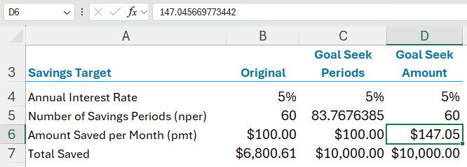
Let’s say your 13-year-old wants to save $10,000 by their 18th birthday to buy a car. They currently save $100 per month in an account that earns 5% interest annually. Let’s calculate how much they will have in 5 years and then use Goal Seek to determine how long they need to save to reach $10,000.

Step 1: Calculate Future Savings Using the FV Function

Excel’s FV Function (Future Value) helps us determine the final savings amount.

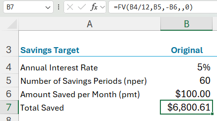
Formula:

=FV(B4/12, B5, -B6, , 0)

Where:

• B4/12 → Interest rate per month (since B4 contains the annual rate)
• B5 → Number of saving periods (60 months)
• -B6 → Monthly savings (negative since it's an outgoing payment)
• 0 → Payments occur at the end of each period

Result: After 5 years, they will have $6,800.61, which is short of the $10,000 goal.

Step 2: Use Goal Seek to Find the Required Saving Period

Now, let’s use Goal Seek to determine how many months are needed to reach $10,000.

1. Copy the calculations to another column so we can compare results.

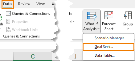
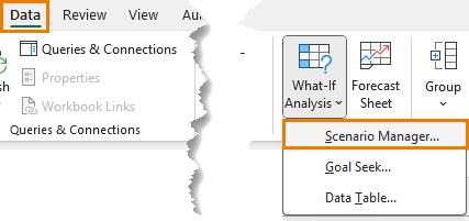
2. Navigate to Data tab > What-if Analysis > Goal Seek.

3. Fill in the Goal Seek fields:

• Set cell: The cell with the future savings formula (e.g., C7).
• To value: 10000 (our target).
• By changing cell: The number of months (C5).

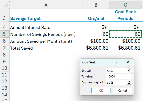
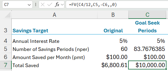
4. Click OK—Excel will iterate and find that 84 months (7 years) are needed to reach $10,000.

Step 3: Use Goal Seek to Adjust Monthly Savings

If the goal is to stick to a 5-year plan, let’s calculate the required monthly savings.

1. Copy calculations to a new column.
2. Open Goal Seek.
3. Set the fields:
• Set cell: Future savings cell.
• To value: 10000.
• By changing cell: Monthly savings amount.

Result: They need to increase monthly savings to $147.05 to reach $10,000 in 5 years.

Example 2: Loan Payments

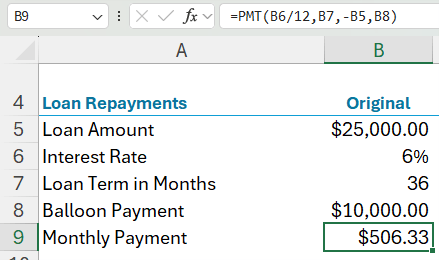
Now, suppose your teen considers getting a loan instead. They plan to buy a $25,000 car with a 6% interest rate over 36 months. Let’s calculate the monthly payment and then use Goal Seek to determine how much they can afford to borrow if they can only pay $400 per month.

Step 1: Calculate Loan Payment Using PMT Function

Excel’s PMT function calculates the monthly loan payment:

Formula:

=PMT(B6/12, B7, -B5, B8)

Where:

• B6/12 → Monthly interest rate (divided by 12)
• B7 → Loan term in months
• -B5 → Loan amount (negative because it’s borrowed money)
• B8 → Balloon payment (final balance due after the loan term)

Result: The monthly payment is $506.33, which is too high.

Step 2: Use Goal Seek to Determine Affordable Loan Amount

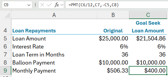
If the budget allows only $400 per month, let’s use Goal Seek to adjust the loan amount.

1. Copy calculations to a new column [optional].
2. Open Goal Seek.
3. Set the fields:
• Set cell: Loan payment cell.
• To value: 400.
• By changing cell: Loan amount.

Result: Goal Seek determines that they can borrow up to $21,504.86 and stay within the $400 budget.

Example 3: Comparing Loan Scenarios Using Scenario Manager

Instead of manually running multiple Goal Seek calculations, we can use Scenario Manager to compare different loan terms and balloon payments.

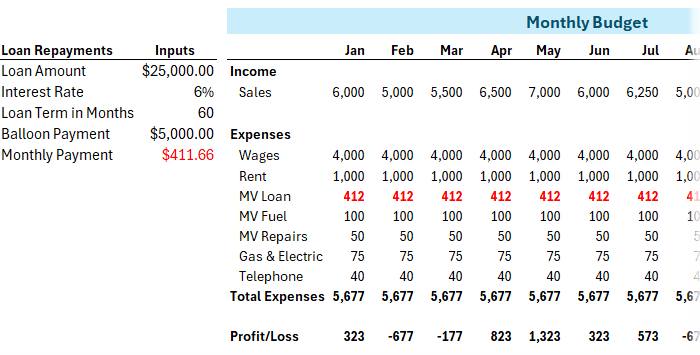
This is handy if the loan repayment feeds into a larger model like the example below where the loan repayment feeds into our monthly budget, and you don’t want to recreate the whole model to compare different scenarios.

Step 1: Open Scenario Manager

1. Navigate to Data tab > What-if Analysis > Scenario Manager.

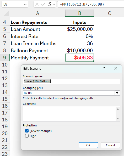
2. In the dialog box, click Add to create a scenario.

Step 2: Create Loan Scenarios

You can create multiple scenarios. I’ll create two:

• Scenario 1: 3-year loan, $10,000 balloon payment
• Changing cells: $B$7:$B$8
• Values: 36 months, $10,000 balloon

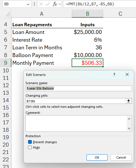
• Scenario 2: 5-year loan, $5,000 balloon payment
• Changing cells: $B$7:$B$8
• Values: 60 months, $5,000 balloon

 

Step 3: Compare Scenarios

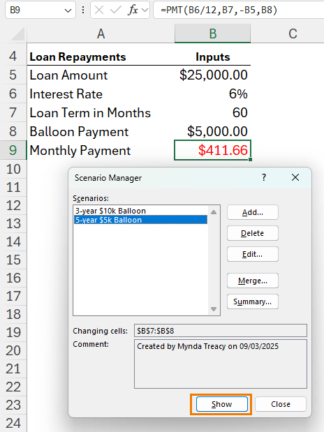
1. Select a scenario and click Show to see the impact.
2. The budget shifts, revealing whether the loan term needs further adjustments.

 

Tip: You can add more scenarios and also look at altering other variables, like the loan amount.

Better Together

With Goal Seek and Scenario Manager, you can replace manual guesswork with precise calculations in seconds and toggle between different options to see the impact on a larger model.

Whether you’re saving for a goal, determining loan payments, or comparing financial scenarios, these tools save time and ensure data-driven decisions.

What Next:  Goal Seek and Scenario Manager are just two of many features that can save you time and frustration. Check out my Excel Expert Course for step-by-step lessons, certification, and personal support.