How to Create a Reverse PivotTable - this is genius.
This tutorial was sent in by Bryon Smedley of Bristol, Tennessee.
There comes a time when you are presented with data in a cross-tabular format but your analysis requires that the data be formatted into a traditional table (or normalized) structure.
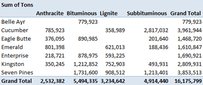
… but you need it to be in THIS format.
How can this be achieved?
The answer is simpler than you may think.
The first thing you need to do is access a tool that, prior to Excel 2007, was fairly easy to reach.
It has now been pushed into the background of Excel 2007 and Excel 2010; that tool is the Pivot Table and Pivot Chart Wizard.
This used to be the de facto standard tool for building Pivot Tables and Pivot Charts prior to the 2007 redesign.
The tool still exists within Excel, you just have to dig a bit to find its hiding place.
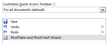
Part A: Load the Pivot Table and Pivot Chart Wizard into your Quick Access Toolbar
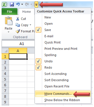
- Click the small down arrow to the right of the Quick Access Toolbar (top left corner of Excel) and select More Commands…
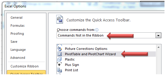
- Click the dropdown arrow next to Choose commands from: and select Commands Not in the Ribbon. This will produce a list of Excel features not located on the Ribbon. Scroll down and select PivotTable and PivotChart Wizard.
- Click the Add >> button in the middle of the Excel Options dialog box.
- Click OK to continue.

This will place the PivotTable and PivotChart Wizard feature in the right column of selected Quick Access Toolbar features.
Part B: Reverse the Pivot
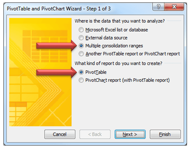
- Click the PivotTable and PivotChart Wizard button on the Quick Access Toolbar
- In Step 1 of the wizard, select Multiple Consolidated Ranges from the top question and PivotTable from the bottom question then click Next >.
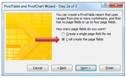
- In Step 2 of the wizard, select I will create the page fields and then click Next >.
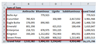
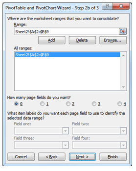
- With your cursor in the Range: field, highlight the area of data you are wishing to convert to a table and then click the Add button. IMPORTANT: DO NOT highlight any total columns or rows that may be to the right or below the data. In this example, the selected data would start in cell A2 and end in cell E9. Finish this step by clicking Next >.
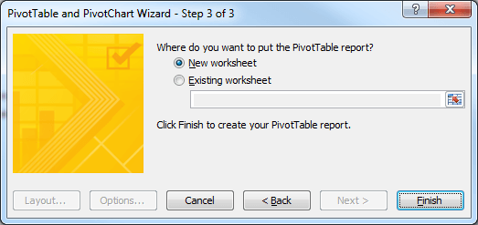
- In step 3 of the wizard, select New Worksheet and then click Finish.
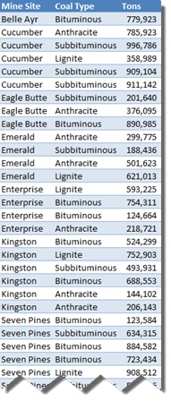
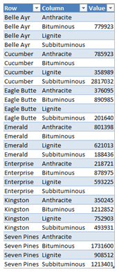
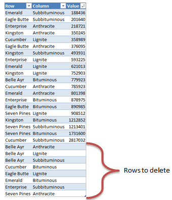
- Double click on the Grand Total number (in this example, the number 20 in the lower right). This will generate your normalized table as seen below.

This will produce a new pivot table similar to the one below. Do not worry about any of the numbers or layout; this is an intermediate step that will be discarded in the end.
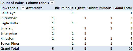
Because not every row category contains a corresponding column category entry, those entries have no values. You can either filter out the “Blanks” or sort the list by value and then delete the rows with no values.
Thanks again, Bryon for sharing your knowledge.
If you use PivotTables you’ll agree that when you come across data in the wrong format it is often a show stopper.
But now, thanks to Bryon’s genius technique, we can easily put the data in the correct format and happily Pivot away!
Bryon is from Bristol, Tennessee and has been teaching Excel since version 7 which was included with Office 95. He is currently a Technical Training Analyst for one of the largest coal companies in the world. His key responsibility is to conduct all Microsoft Office training, but in addition he also serves as a technical consultant for any and all projects involving Microsoft Office applications.
Bryon says “Excel is by far my favorite among all the Office applications due to the almost infinite number of situations it can be used. There literally seems to be no end to its usefulness.
My favorite Excel tools are difficult to narrow down. Without getting into third party add-ins, I would have to say PivotTables (especially with the addition of Slicers. WOW! Are those things awesome!!), the Text to Columns tool (what a time saver), and Macros.”
Vote for Bryon
If you’d like to vote for Bryon’s tip (in X-factor voting style) use the buttons below to Like this on Facebook, Tweet about it on Twitter, +1 it on Google, Share it on LinkedIn, or leave a comment….or all of the above 🙂
I’ll do a tally at the end of the competition and announce the winner!

thanks, the descriptions was definitely clear. i should say these “Full REVERSE”
looks like dsum to me, thank you Gm
Not sure what you’re referring to, Wilson.
This is so helpful – thank you so much…
Glad you liked it, Fran 🙂
Thanks Mynda and Byron
This is an amazing tip. I am going to start using this. Never knew this could be done.
Thanks, Virendra. Glad you found it useful.
Mynda
This is fantastic except for text fields. Why do text fields not come back as text? I had text fields in Row Labels but with reverse pivot I get only 1s and 0s.
Also, saw a comment re: not having the options you mention above when starting. If cursor is in the PT, you can only create another PT. Place cursor outside of PT to get options.
Thanks for a great website!
Hi Dana,
It should work for text fields too, just as the example has text in the first column. Are you able to send your workbook in so we can take a look what you mean?
Mynda
It is excellent. I searched on internet for many many hours until I found your article. You solved the exact same problem I have.
Thank you very much for sharing this technique!
Glad you found it useful, Kai. You might also like to check out Power Query for unpivoting.
Dear Mynda,
The “reverse pivot table” technique to create a “real” pivot table is a terrific technique.
I suspect consolidation option was originally intended to actually combine multiple ranges into a single PT report.
Yet, I never see an example of this. Can you explain the usage of the four separate Page Fields?
Thanks.
Hi Philip,
You’re right, consolidation is for creating a PT from ranges from multiple sheets.
You can use those Page fields to add a label to identify each added range. If you consolidate data from 4 sheets, you can label each range with a relevant name, these labels will be added to Report Filter field of the consolidated pivot table.
Cheers,
Catalin
Brilliant tip Bryon! Im going to use it now!!! Thanks for the recco Mynda 🙂
This is just sensational, thank you.
Wonderful! Glad you liked it 🙂
Wow! I had no idea this was in Excel (2010).
Glad you liked it, Bob 🙂
This worked really well for me till Excel 2007 – so many many thanks!!
In Excel 2013, the Pivot Table wizard no longer provides the option for “multiple consolidated ranges”.
So in order to be able to use the same trick as above in Excel 2013, the only thing that we have to change is the way we call up the Pivot Table wizard. Instead of adding it in the Quick Access Toolbar, just use the good ol’ shortcut : Alt + D + P.
This opens up the Pivot Table wizard, with the Multiple Consolidation ranges option.
Credit: https://www.youtube.com/watch?v=N3wWQjRWkJc
Hi Maya,
I have the PivotTable Wizard in my Excel 2013 QAT and it gives the option for Multiple Consolidation ranges so I’m not sure why you think it doesn’t work the same.
ALT+D+P is simply the short cut keys which open the PivotTable Wizard, just as the icon does.
Mynda
Very valuable and simple trick.
cheers, Satish.
This was worth the price of admission. I can redo so much because of this.
Great trick and thanks for posting.
🙂 cheers, Grant. That is one of my favourite tricks too!
That was awesome! Thanks so much. I’ve been struggling with this for a few hours; your instructions were perfect!
Cheers, John. Bryon’s tutorial is one of my favourite Excel gems too 🙂
Great and anyone can learn who want to learn
🙂 Indeed, Mukesh. I hope you find our site helpful.
Kind regards,
Mynda.
This tip just saved me half an hour work every week! Purely amazing trick!!!
🙂 Awesome, Heikki. Glad we could make such a difference for you.
Here I am, still learning after all these years and versions of Excel 🙂
Very good!
Duncan
Glad you liked it, Duncan 🙂
Hi Mynda,
I’ve been looking for a solution like this for sometime, not knowing how simple it could be, ironically it was right there within Excel all along. Thank you, thank you, thank you……
I came across a VBA solution (UnPivot) by Jeff Weir that does the work nicely, but yours requires no coding.
And thanks again, keep up the good work.
Pablo
Cheers, Pablo. Thanks for sharing Jeff’s link. Glad you also liked the non-VBA solution 🙂
i have no idea how to create a pivot table from scratch assist
Hi Blessed,
You can find tutorials on creating Pivot Tables here.
Kind regards,
Mynda.
This is extremely helpful, thank you very much.
Cheers, Steve 🙂 Glad you liked it too.
Great information and you have a great web site, Mynda!
Using a pivot table and the data in your example, I summed the data under the column headings. By adding Anthracite, Bituminous, etc. to the “Sum of Values” area of the Pivot table, under “Column Labels” in the Pivot table a “Sum of Values” appears, as “Sigma of Values.” By dragging this field to the Row Labels of the Pivot table window, under the column label I called “Type” (for Belle Ayr, Cucumber, etc.) the same result occurs, only with “Sum of” Anthracite, etc, which can easily be changed.
I used this method to turn 5,000 rows of aggregated data into 88,000 distinct records I could then analyze using a new pivot table.
Thanks again for your web site.
Awesome result! Thanks for sharing, Gary 🙂
Bryon’s reverse PivotTable tip was my favourite out of the Excel Factor series.
And thanks for your kind words about our site.
Brilliant. An excellent tutorial.
Cheers, Andrea. That’s one of my favourites too 🙂
Thanks very nice blog!
Thanks, Bou 🙂
Excellent tutorial! Simple, clear steps that anyone can understand. THANX
Hi Ravi,
On behalf of Mynda,
You’re welcome!
Cheers,
CarloE
Great tutorial for new users to MW 2010. Step by Step was a big help! Thanks.
Hi Nat Marie,
On behalf of Mynda,
You’re welcome.
Cheers,
Carlo
This worked perfectly. I had created an order entry sheet with the name running down the left and the items going across the top. Calculations to figure out people and product totals. I needed to reverse the pivot style for a simple list of names and items ordered.
Thanks for the post!!!
Got it. very nice.
Hi Mynda,
Hope you are doing good….
Here i am, again looking for your assistance Mynda, I have few basic queries regarding excel…
1) I have excel sheets with data upto 800000 rows and around 52 columns, how will you term it in matter of Size i.e huge and what function we can use in order to derive report.
2) Can we use Pivot in one workbook while data in other workbook. Is there any demerits of it…
3)Can we use Pivot in excel while data stored in Access. If yes then is there any Demerits we have or points we need to take care of.
4) Is there any way we can have Dynamic Pivots, here i mean can we make Pivot table have dynamic range.
Thanks
Minku
)
Hi Minku,
In each case I would use a PivotTable to analyse the data. One of the downsides of PivotTables is they’re restrictive in their formatting to a degree. Yet with the volume of data you have it would still be your best option. I would format the data as a Table, this will mean the PiovtTable automatically picks up the new data added to the bottom of the table.
You can read about how to set up your PivotTable so that it automatically refreshes here.
You might also be interested in learning my Power Pivot course
Kind regards,
Mynda.
Hi Mynda,
the trick can be expanded if you have more than 1 dimension in the header rows.
Example:
Row A: June June July July
Row B: Budg Actu Budg Actu
First you create a concatenated name (B1 & “;” & B2) with a separator character (semicolon, paragraph, or anything that will not occur un your headers…) in a new row (e.g. row 3).
Then you calculate the pivot starting with row 3. At the end all you need to do is Data->Text to columns applied on the concatenated name.
Hi Wolf,
Great tip. Thanks 🙂
Mynda.
Beautiful tip for excel tables and pivot table use
Clear and simple tutorial…..
Excellent tutorial! Simple, clear steps that anyone can understand. Genius? Agreed.
Thanks, Angie. Glad you liked it 🙂