Excel Factor 21 Hyperlink Triptych

These Excel Factor tips were sent in by Zoran Stanojevic of Belgrade, Serbia.

Words by Mynda Treacy

Zoran has prepared 3 distinct ways we can apply hyperlinks that dynamically update depending on the selection we make.

The selection can be controlled with either a data validation list or a spin button form control.

Download the workbook.

Warning! These are advanced tips. I am not going to do step by step instructions to the extent that I usually do.

Instead I’m going to focus on the unique aspects of Zoran’s work and allow you to download the workbook to see ‘under the bonnet’ to fully understand the intricacies.

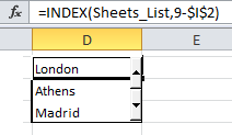
1. Hyperlink with Data Validation

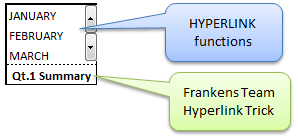
This first example is a hyperlinked data validation list. Zoran learnt this tip from the Frankens Team, and you can learn how to wrangle Excel to allow you to insert a hyperlink to a dynamic named range used in a data validation list here on their blog.

Bonus tip:

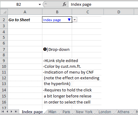
One of the downsides of data validation lists is the down arrow indicator only appears if the cell is selected.

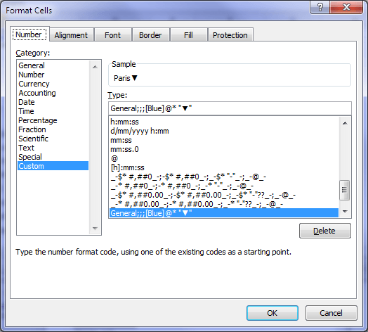
To overcome this Zoran has added a custom number format to the cell containing the data validation list so that it shows an upside down triangle symbol appended to the sheet name, plus it displays the font in blue, the default for a hyperlink.

The Downside of Hyperlinks with Data Validation

You need to use either your arrow keys to navigate to the cell, or Go To (CTRL+G), or click and hold the mouse until the fat cross appears. Otherwise you execute the hyperlink.

The next 3 examples are variations of one another.

2.1 Spin Button with Hyperlink 1

Features:

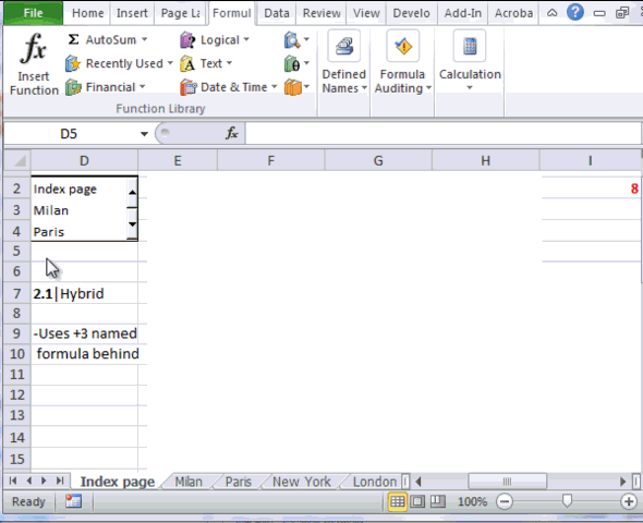
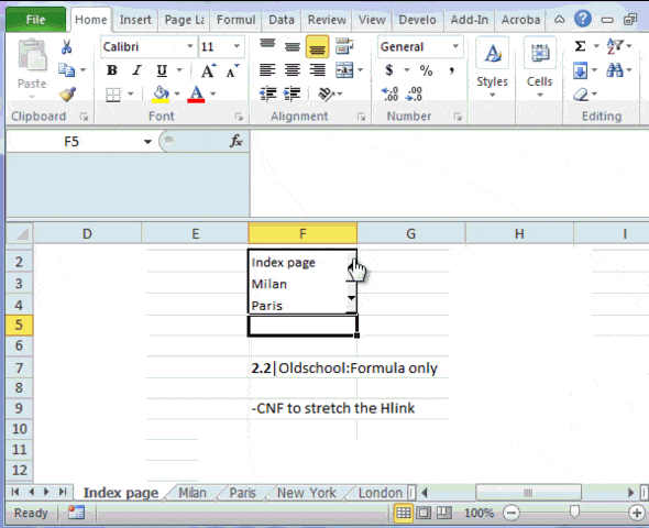
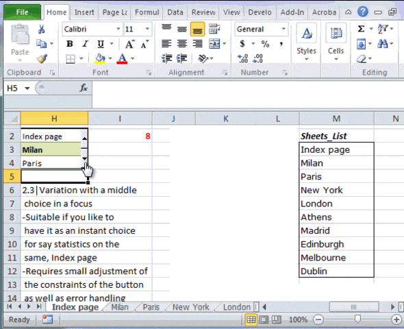
A spin button form control manages the selection.  The form control output is in cell I2 and has a minimum value of 1 and maximum value of 8.

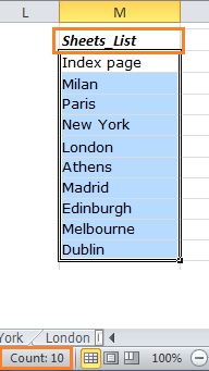
Below are the cells that make up the named range ‘Sheets_List’. You can see from the count indicator that there are 10 items in the list.

An INDEX function returns the sheet name from the ‘Sheets_List’ with these formulas:

Cell D2

=INDEX(Sheets_List,9-$I$2)

Cell D3

=INDEX(Sheets_List,10-$I$2)

Cell D4

=INDEX(Sheets_List,11-$I$2)

The hyperlinks are managed using 3 separate named formulas; one for each item visible in the list. Scrolling through the list changes the form control output in cell I2 and dynamically updates both the name displayed in the list and the hyperlink.

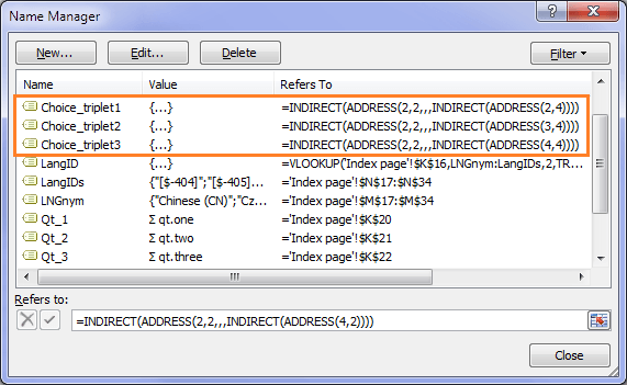
To insert the named formulas you need to use the Frankens Team hyperlink trick mentioned in the first example above.

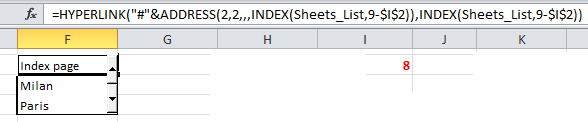
2.2 Spin Button with Hyperlink 2

Unlike the previous example, this uses the HYPERLINK function to create the dynamic links:

You can read more on the HYPERLINK function and the use of the # symbol here.

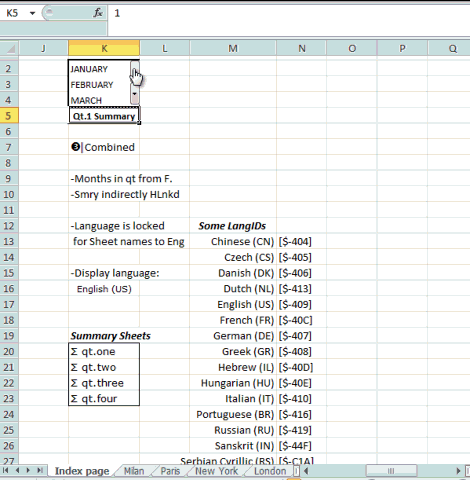
2.3 Spin Button, Hyperlink and Cell Formatting

This uses some simple cell formatting to draw attention to the middle choice.

The spin button control settings have a minimum value of 0 and maximum value of 9, as opposed to 1 and 8 respectively for the previous 2 examples. As a result, the formulas for each choice are slightly different to handle errors:

Choice 1:

=IF($I$2<9,HYPERLINK("#"&ADDRESS(2,2,,,INDEX(Sheets_List,9-$I$2)),INDEX(Sheets_List,9-$I$2)),"")

Choice 2:

=HYPERLINK("#"&ADDRESS(2,2,,,INDEX(Sheets_List,10-$I$2)),INDEX(Sheets_List,10-$I$2))

Choice 3:

=IF($I$2,HYPERLINK("#"&ADDRESS(2,2,,,INDEX(Sheets_List,11-$I$2)),INDEX(Sheets_List,11-$I$2)),"")

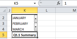
3 Spin Button List Hyperlink and a Zillion Other Tricks!

This is the Full Monty!

Like the previous examples, this also uses a Spin Button, but because quarterly groups of months are displayed, the formula behind each month is unique:

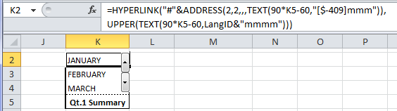
Cell K2:

=HYPERLINK("#"&ADDRESS(2,2,,,TEXT(90*K5-60,"[$-409]mmm")),UPPER(TEXT(90*K5-60,LangID&"mmmm")))

Cell K3:

=HYPERLINK("#"&ADDRESS(2,2,,,TEXT(90*K5-30,"[$-409]mmm")),UPPER(TEXT(90*K5-30,LangID&"mmmm")))

Cell K4:

=HYPERLINK("#"&ADDRESS(2,2,,,TEXT(90*K5,"[$-409]mmm")),UPPER(TEXT(90*K5,LangID&"mmmm")))

How to calculate a date using the TEXT function

First let’s understand how the month is derived for the link_location argument of the HYPERLINK Function.

Remember the spin button output is in cell K5 (currently containing 1) and the first TEXT function is evaluating the month name.

Using cell K2 as our example:

=HYPERLINK("#"&ADDRESS(2,2,,,TEXT(90*K5-60,"[$-409]mmm")),UPPER(TEXT(90*K5-60,LangID&"mmmm")))

Step 1: TEXT(90*1-60,"[$-409]mmm")

Step 2: TEXT(30,"[$-409]mmm")

Step 3: TEXT(30/01/1900,"[$-409]mmm")

Step 4: TEXT(Jan)

Hint: if you type the number 30 into a cell and format the cell as a ‘short date’ it will display 30/01/1900 or 01/30/1900 if you use mm/dd/yyyy format.

That's because all dates and time in Excel are given a serial number. The serial number for 30th January 1900 is 30.

The [$-409] forces it to always evaluate in English. This is because the worksheet tab names are in English and this part of the formula is returning the address for the hyperlink.

The ‘mmm’ formats it to the first 3 letters of the month name (again, because all of the worksheet names are only the first 3 letters of each month).

So, what about the other months…

February:

Step 1: TEXT(90*1-30,"[$-409]mmm")

Step 2: TEXT(60,"[$-409]mmm")

Step 3: TEXT(29/02/1900,"[$-409]mmm")

Step 4: TEXT(Feb)

March:

Step 1: TEXT(90*1,"[$-409]mmm")

Step 2: TEXT(90,"[$-409]mmm")

Step 3: TEXT(30/03/1900,"[$-409]mmm")

Step 4: TEXT(Mar)

As the spin button output value in cell K5 increases the month dynamically updates.

How to Translate Language

Now we’ll look at the second TEXT function used for the friendly_text argument of the HYPERLINK Function to understand how Excel can translate languages.

Again using cell K2 as our example:

=HYPERLINK("#"&ADDRESS(2,2,,,TEXT(90*K5-60,"[$-409]mmm")),UPPER(TEXT(90*K5-60,LangID&"mmmm")))

We already know how the first part evaluates the date from the previous example so we’ll focus on the translation.

Step 1: TEXT(90*K5-60,LangID&"mmmm")

LangID is a named formula:

=VLOOKUP('Index page'!$K$16,LNGnym:LangIDs,2,TRUE)

Named ranges LNGnym and LangIDs used in the above formula are the two columns of the Language ID’s table below. K16 is the data validation list for the language choice.

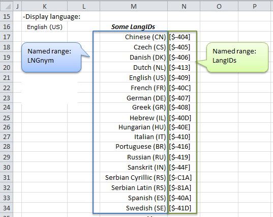
Is your language missing? Click here for a complete list of language ID numbers.

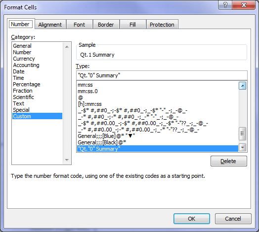
Custom Number Format

Again, Zoran has used a clever custom number format to display the spin button output with some meaningful text:

More on custom number formats in this comprehensive Excel custom number format guide.

Dynamic Hyperlinks

This example incorporates two techniques for the hyperlinks.

The months use the HYPERLINK Function, and the 'Qt.# Summary' in cell K5 uses the Frankens Team trick.

UPDATE: Zoran has made some improvements on examples 2.1 and 2.2 above which simplify them.

Thanks for sharing your ideas with us, Zoran.

“My name is Zoran and I am from Serbia. I have worked with Excel since my first employment back in 1996 (Office 97) and I was immediately drawn to VBA. Although my main expertise was wider IT administration, Excel Macro/VBA development gets an ever bigger share.

Serbians have many ethnicities and all have rights to use their own language (including the alphabet) in formal communication with the public services as well as through formal education. Serbia itself has two alphabets: Latin and Cyrillic and apart from that, in the Autonomous Province of Vojvodina another 5 official languages exist.

In January I moved back to my hometown Subotica where I work in the City Administration IT department. This year I was involved in the preparation processes for the Serbian elections in my municipality, where I took part in data mining and reporting during and after the elections. It was challenging since elections were held on all levels: both parliamentary and presidential, for the state, autonomous province, districts and down to the very cities and towns.

The City Administration in Subotica has one of the most efficient and best organized public services in the country and the IT Department is the skeleton of the system, so it is a great experience to work here, and be part of it.”

Vote for Zoran

If you’d like to vote for Zoran's tips (in X-factor voting style) use the buttons below to Like this on Facebook, Tweet about it on Twitter, +1 it on Google, Share it on LinkedIn, or leave a comment to thank Zoran for taking the time to suggest this tip….or all of the above 🙂