This Excel Factor tip was sent in by Bob Cooke of Lincolnshire, England.
Words by Mynda Treacy
Last week Bob emailed me with an example of how he uses the INDEX, SMALL, IF and ROW functions to lookup a list and return multiple matches like this:
It’s good timing as I actually had this on my To-do List to write about once I ran out of Excel Factor entries.
How to Lookup and Return Multiple Matches
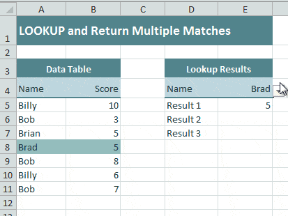
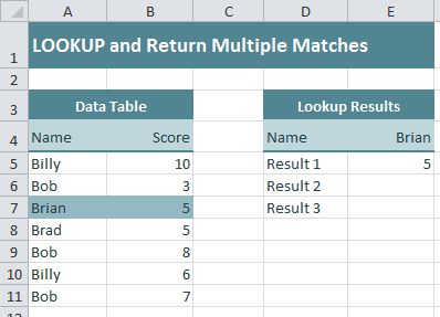
Let's take the example below where we want to find the 3 results for Bob.
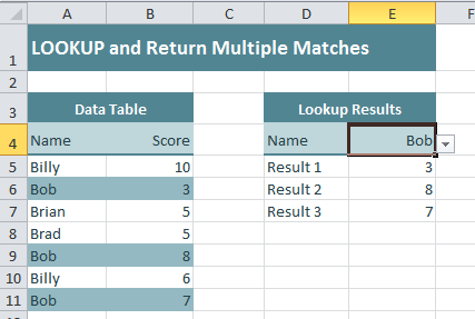
We can use the array formula below in cell E5 to look up our Data Table (cells A5:B11) and return the first result that matches the value in cell E4:
=IFERROR(INDEX($A$5:$B$11,SMALL(IF($A$5:$A$11=$E$4,ROW($A$5:$A$11)-4),ROW(A1)),2),"")
Because it is an array formula you need to enter it with CTRL+SHIFT+ENTER.
We can then copy the formula down to cells E6 and E7, which is as many as we need since there are a maximum of 3 results for any one person in the list.
When we copy the formula down the ROW(A1) reference will update to ROW(A2) and so on, and as a result it will return the 2nd, then the 3rd result….more on that later.
Evaluating the Formula
Essentially we’re using an INDEX function to lookup the name in cell E4 in the range A5:B11 and return the values in column B that correspond to Bob.
Remember, the INDEX Function returns a value at the intersection of a particular row and column in a given range.
The syntax for the INDEX function is:
=INDEX(array,row_num,[column_num])
In this formula we’re employing the help of SMALL, IF and ROW to complete the row_num argument.
Step 1 – IF Function
The IF Function checks to see which values in cells A5:A11 = Bob, and then returns the row numbers that match.
Rows 2, 5 and 7 contain the name Bob (that is the row numbers in the range A5:A11, not the worksheet row number. Hence the minus 4 in ROW($A$5:$A$11)-4) which accounts for rows 1-4 that aren't part of our range.)... so, our formula now looks like this:
=IFERROR(INDEX($A$5:$B$11,SMALL({2,5,7},ROW(A1)),2),"")
Step 2 – SMALL Function
The SMALL Function returns the k-th smallest value in a data set. The syntax is:
=SMALL(array,k)
Where k is the position in the array to return.
And, since the ROW function returns the row number of a reference, ROW(A1) evaluates to 1, therefore our SMALL formula is:
SMALL({2,5,7},1)
And evaluates to 2, i.e. the smallest value in the array.
Now our formula looks like this:
=IFERROR(INDEX($A$5:$B$11,2,2),"")
And in English it reads:
Lookup the range A5:B11, find the value at the intersection of the 2nd row and 2nd column, if there is an error; return nothing.
Remember when we copy down the formula to cells E6 and E7 the ROW argument changes to ROW(A2) and ROW(A3) respectively. As a result our SMALL formula evaluates as follows:
Cell E6: SMALL({2,5,7},2)
And:
Cell E7: SMALL({2,5,7},3)
Step 3 – INDEX Function
Handle errors with the IFERROR function.
If we didn't use IFERROR and we selected a name that only has 1 or 2 results we would get an ugly #NUM! error. Instead, with IFERROR we can instruct Excel to leave the cell blank. I think you'll agree cells E6 and E7 below look nicer blank:
Alternatively you could replace blank with N/A or similar if you prefer.
Enter your email address below to download the sample workbook.
Thanks to Bob for suggesting this tip.
Bob has worked in heavy engineering in the steel industry for over 40 years.
"For the later part of my career I have been using AutoCAD for design. I have for the past three to four years been using excel for minor “filing” purposes. I have in the past 8 months started to explore excel and have realised that there is a very powerful programme not being used so I am studying as much as I can."
Vote for Bob
If you’d like to vote for Bob’s tip (in X-factor voting style) use the buttons below to Like this on Facebook, Tweet about it on Twitter, +1 it on Google, Share it on LinkedIn, or leave a comment to thank Bob for taking the time to suggest this tip….or all of the above 🙂
I have tried to get the list of 5 person with same birth date thru VLOOKUP option but system is repeating the first name of the list in all 5 rows. Please advise
Hi Shaikh,
This article provides an INDEX-SMALL solution, try this one instead of VLOOKUP. You can download the sample workbook to try it.
Hi,
I am currently using this formula in an ‘Items Received’ spreadsheet. While it works when entering one Purchase Order Number in Column A to return all related items, can I then enter a second Purchase Order in Column A to return those items?
Hi Shane,
I’d just use a PivotTable to filter the data so it returns the details for the Purchase Orders you want. Formulas are just making hard work for yourself.
If you’d like some help on how to use a PivotTable for this, please post your question in our Excel forum where you can upload a sample Excel file.
Mynda
I have been working on this for days and have tried using the same syntax as this with just blank results. I want to list all of my students on one sheet and have them populate on the right class sheet automatically if they are in that class. This shouldn’t be that hard! Can you tell me what I am doing wrong?
Hi Heather,
Please post your question and sample Excel file on our Excel forum so we can see what you’re doing and help you from there.
Mynda
How do we extend this for multiple criteria? Something like:
Return a list of all students in with “B” in the Group Column, and have a “Yes” in the Absent Column?
Hi Mike,
I wouldn’t use a formula at all. This is what PivotTables can do in a snap, with no complicated formulas. If you’re not sure what to do, upload a sample Excel file to our Excel forum and we’ll provide you with an example.
Mynda
Can any one help me to shift the row from B to C,……….
Hi Mohamed,
Not sure what you want to do, B and C are columns, not rows.
Select the entire row (or column), – choose Cut from right click, then select the position where you want the data to be and press Ctrl+Shift+=, it will insert the range you cut.
I have played with this formula for the better half of the day, it will only return the 1st array of data in the data set regardless of the match and will not return a list of matches. What am I doing wrong? I have tried to replicate your exact data set in the exact cells and copied and pasted the exact formula, and although I select Bob, Result 1 is showing up as 10 – the first return of the data set and does not match E5. Uggg, beyond frustrated!!
I am using MacBook Pro and the newest version of excel.
Hi Joann,
We have to see what you did to tell what’s wrong. Can you upload your file on our forum? (create a new topic after sign-in)
Hi,
As it’s an array you need to type in the formula and then (on a mac) press cmd+Shift+Enter, this will then add {} either side of the formula and voila.
if you change the formula to pick up different cells etc you will need to remake this an array by doing the cmd+shift+enter.
Hope this helps if you have not sorted it
Hi.
This one is such a big help.
But how would it look it the lookup data is in another file?
I’m asking since I can find another use for this at my company where I have my pricelist in an external file, but still need the multiple results in a collum
Hi Daniel,
You should setup a connection to that file, to bring data in. Usually, power query is the tool for this. More, if you use power query, you might not need formulas any more, the lookup can be performed within PQ.
Catalin
Using a second column as a unique identifier, is there a way to take a column of data consisting of positive and negative numbers and offset the values with the fewest number of matches?
Example:
Column A – Account # (unique identifier)
Column B – Outstanding Balance (numerical value positive or negative)
Returning the information to columns C & D, with column C as the Account # (identifiers) and column D the numerical values that offset each other.
Basically, I’m looking for a formula to match and offset volumes in the most efficient manner. As the offset will be entered manually. Any help is much appreciated. Thanks!
Hi Andy,
Can you please create a new topic on our forum? You have to prepare and upload a sample file so we can see your data structure, it will be easier to understand what you need.
Thanks
Catalin
I was wondering if there was a way to lookup one search field using this function, format, from a different spreadsheet within the book, but when it finds what was called, it copies all corresponding data from that row in where the code syntax is underneath it
ie ={IF(ISERROR(INDEX($A$1:$B$8,SMALL(IF($A$1:$A$8=$E$1,ROW($A$1:$A$8)),ROW(1:1)),2)),””,INDEX($A$1:$B$8,SMALL(IF($A$1:$A$8=$E$1,ROW($A$1:$A$8)),ROW(1:1)),2))}
but how would I modify that to allow it to access data from a different spreadsheet within the same book and copy the whole row not just the one result?
-Thank you
You can’t do that, if you want to return results from multiple columns, same row, you have to set formulas in each cell, each should return values from the corresponding column.
If you open a new topic on our Forum with a sample file and details of what you need to do, we will help you find a way to do that.
Catalin
Hello
I need help! I need a formula to add up all the same names of suppliers in a separate sheet. I can’t seem to figure it out
Thanks
Hi Jan,
You can use SUMIF or SUMIFS for this.
You can post a question in our Excel Forum if you get stuck.
Mynda
Hi, I need help on my formula. I need multiple number’s from one column on sheet 1 to be returned to a row in sheet 2. What I can’t get right is to transfer the cells that meet the criteria in merged cells in sheet 2 from A1:H1. I basically need the information to be transferred starting from I1. For some reason when I change the formula column part to 5, the cells get repeated two or three times. Here is the formula I’m using;
{=IFERROR(INDEX(SHEET1!$H$1:$H$300,SMALL(IF(SHEET1!$G$3:$G$300=$A1,IF(SHEET1!$F$3:$F$300=1,ROW(SHEET1!$G$3:$G$300),””)), COLUMN ()/5)),””)}
Can you please assist me.
Hi Vinette,
Can you please upload a sample file with your formula on our forum? (create a new topic). It’s not easy to understand what’s wrong without seeing the data. Why are you using COLUMN()/5 in the second argument of the SMALL function? That argument expects integers, not fractional units.
Catalin
Hi,
I have question:
I want to match company names list with employees list for more than one employee name
I tried Vlookup and it gives me only one employee name per company.
=Vlookup(B1 company name, A:C range, 2, False)
Also, I used Index, match:
=index(A:A range of emloyees,Match(B1 company name, C:C range of company names in the other excel, 0))
But it didn’t work either and it gives me the same result (only one employee per company)
Anyone can help please?
Hi Sam,
It’s difficult to say based on this information. Please post your question on our Excel Forum and include a sample Excel file with some of your data, or dummy data, and we’ll take a look.
Mynda
Hello good evening,
I need small help. So I need to get how many same numbers repeats in Column A that matches same value in column B. Example How many times 38692 repeats in column A and has value of $5 in column B? Can anyone help me with that please?
A B
38770 $10.00
38692 $5.00
38692 $5.00
38692 $5.00
38692 $10.00
38769 $10.00
38692 $5.00
38692 $5.00
38692 $10.00
$0.00
$0.00
38694 $10.00
$0.00
38694 $10.00
$0.00
Hi Joseph,
It’s a simple COUNTIFS:
=COUNTIFS($A$1:$A$15,A1,$B$1:$B$15,B1)
Put this formula in column C.
Cheers,
Catalin
Hello,
I need to do something similar, but total the amounts in column B if they repeat in column A.
Example
38694 totals to $20.
Hi Finch,
Can you please post your problem with sample data and description to our forum? (create a new topic after sign-up) It will be easier to help you.
Regards,
Catalin
I believe I understand everything except, how do highlight the Name/Score row upon name selection with the drop down list? I believe I could use a macro or VBA but I can’t figure out how you’re doing it.
Hi Robert,
I used Conditional Formatting to highlight the selected name. Here is a tutorial on Conditional Formatting with formulas
And if you click here to download the workbook from this tutorial then you can see how I set it up.
Let me know if you get stuck.
Kind regards,
Mynda
I have lowest price from many offers that quoted from different suppliers. Now I want to pick up the name of supplier that offered lowest offer and second lowest offer and third offer with supplier name from the worksheet. Can you assist in this? pls help
Hi,
Can you please upload a sample workbook with your data structure on our Help Desk? (create a new ticket). It will be a lot easier to help you if we see your data structure.
Cheers,
Catalin
Seems to be highly interesting
Why when I add a row before the table the function doesn’t work anymore ?
Hi Leandro,
You have to adjust the ranges in formula, they are not dynamic, they are referring strictly to $A$5:$B$11 range. If you need more help, you can open a new ticket on Help Desk, with your test file uploaded.
Cheers,
Catalin
Hi ..thanks for the wonderful solution .. however, there is a big limitation to it as we have to know beforehand how many matches are we going to see ..is there anyway it can automatically detect the number of matches and populate them accordingly ..
Hi Aditya,
Yes, with a PivotTable. Simply analyse the Data Table in a PivotTable to get a summary. In fact you could use the PivotTable for the whole job :-)…but then we wouldn’t have any fun with formulas.
Kind regards,
Mynda
Thanks 🙂 and a Happy new year
Hello Bob,
I really enjoy your Excel articles that are very technical and useful.
I have a particular problem below and would like to ask for your help.
Instead of looking-up and returning multiple matches for one single entry, I would like if it can do for multiple entries given from an input list on one column or separate worksheet.
To output the results, each row will show the matching entry and its matching values can be listed on the next column and/or next column as many as the matching values are found.
And it keeps posting on the next matching entry in the second row and so on for the next.. until all given entries in the list are exhaustedly looked up.
Thanks so much for your help, Bob.
V/r
Tim
Hi Tim,
I’d use a PivotTable and Slicers for this task. I’m sure you could do it with formulas too, but seems like a lot of hard work when a PivotTable and Slicer will do the trick nicely.
https://www.myonlinetraininghub.com/ill-have-a-slicer-that
Mynda
Hello Mynda,
I have rarely used of functions PivotTable and especially new Slicers in my Excel works but definitely will explore these options to resolve the problem.
Thanks Mynda.
Tim
Hi Tim,
Glad you like the look of Slicers and PivotTable functions. Let me know if you get stuck.
Mynda
I’m trying to use this formula to automatically sort mice from one list by cages. I can get it to work for the first cage table (cage 1), but when I try and recreate the formula for another cage table (cage 2) I get nothing (error if I remove the IFERROR condition). If i try and break the formula down, the IF value will only generate a result if the reference cell reads 1, however the original cage table works with any value (so long as it’s in the mouse table). The formula seems to break down completely once I get to the SMALL segment of the formula (if it makes sense to check it that way)…
Hi Eric,
Can you please upload a sample file to our Help Desk? It’s almost impossible to diagnoze without seeing the patient 🙂
Thanks for understanding,
Catalin
Hello,
Instead of only having one column of data as in the example I have 4, how could I select the column that I want return information from?
Thanks,
Hi Maria,
In this formula:
=IFERROR(INDEX($A$5:$B$11,SMALL(IF($A$5:$A$11=$E$4,ROW($A$5:$A$11)-4),ROW(A1)),2),"")The data table has 2 columns:$A$5:$B$11, and the data is returned from column 2 (this is the value for the column argument of INDEX function).
You can have a data table with any number of columns you want, just make sure that the data to be matched is in first column, and change the column argument for INDEX function to your desired column number.
Catalin
Hello Sir,
I have a list of states,city,assessment rates in excel .. The solution i want for this is , in a dropdown box if i select the state , it should load the cities of that particular state and then when i select the state it should give the max assessment rate of that city by comparing for ex:
State city assessment rate
New York New York west 38.23
New York New York east 28.20
New York New York north 20.36
New York New York south 42..23
New York New York 35.55
If i enter new york in dropdown box it should give the max value by comparing all values
Thanks
sorry their’s a mistake in above line.. if select state it should load cities of that particular state and then if i select city it should display the max value of that particular city
Hi Shaan,
Please upload a sample file with details to our Help Desk System, it’s easier for us to work on a file instead of a description.
If you prefer a general solution, then the solution is to use OFFSET in a defined name to create the range for that city only, for the second dropdown.
Catalin
I have a data which are having dates, i want to get the invoice no’s for the dates which are falling under the given week, please help.
Hi Sunil,
Please upload a sample file with details to our Help Desk, it’s a lot easier to work on a real example.
Thanks
Catalin
Thank you very much for this information! Is there a way that we can search for a partial match? (ex. search for “peanut” and receive peanut butter, roasted peanuts, etc)
=INDEX(List!$C$4:$H$200,SMALL(IF(List!$C$4:$C$200=Search!$C$33,ROW(List!$C$4:$C$200)-3),ROW(A1)),6)
Hi Melinda,
Try this array formula (i made a small change to the original formula):
Confirm it with Ctrl+Shift+Enter
It should work fine with partial matches.
L.E:
To use this formula in excel 2003, you can use this version of the formula:
Cheers,
Catalin Bombea
I have lowest price from many offers that quoted from different suppliers. Now I want to pick up the name of supplier that offered lowest offer from the worksheet. Can you assist in this? pls help.
Hi Sabu,
You can test this formula:
Column B in this formula must be Supplier’s Names column, column D must be the list of prices.
Note that if multiple suppliers have the same minimum price, the formula will return only the first supplier with the minimum price.
Catalin Bombea
This is great, thank you!
Does this also work for a Table with named columns instead of A1 refs?
Cheers, Jim. Yes it will work with any reference style.
Kind regards,
Mynda.
I love this tutorial, thank you so much!
I still have an issue and I hope you can help, possible with a VBA code.
How do I insert new row for every match found? In your example you created several rows below for it. Can new rows be inserted with the multiple values?
Hi Eugene,
All you need is to copy down the formula from cell E7, as long as you need, if you think you will have more matches.
Catalin
This article is very helpful. One question, though – I need to be able to sort the data that is returned by the formula (in your example, the results in column E). Is there a way to modify the formula to sort as well?
Thank you!
Hi Betania, the formula for sorting is quite different and complex. The most easiest way to have the results sorted in any way you want: ascending, descending, is to select the data table A4:B11, then sort it by Score, smallest to largest, or largest to smallest; you’ll see that the results will be sorted. If this method is not satisfying, let me know; i’ll work anyway on a solution like that, maybe it will be useful for our members.
Catalin
Unfortunately, the formula is pointing to a pivot table and with the way it’s set up, I am not able to sort it for the columns I am using. I tried different methods of combining the above formula but I could never seem to wrap my head around how it should be put together in order to work. If you can help, I would appreciate it. If not I’ll try to find some other workaround.
Thanks!
Hi Betania,
Can you please send us your workbook so we can see what you’re working with and give you a tailored solution. You can log a ticket in the Help Desk and attach your workbook there.
Thanks,
Mynda.
((IF($A$5,ROW($B$11),ROW($K$11))-ROW())*10+
ABS(IF($A$5,0,COLUMN($K$11))-COLUMN())-
IF($A$5,COLUMN($B$11),0)+1)<=$M$3
Request you to explain me the above formula.
Hi Raghuram,
Let’s take this formula piece by piece:
1.IF($A$5,ROW($B$11),ROW($K$11))
The formula is checking cell A5, if this is TRUE (1) , returns ROW($B$11), if it is FALSE or (0), it will return ROW($K$11);
this is a nonsense, because, no matter if A5 is TRUE (1) or FALSE (0), the result of this formula will be 11, ROW($B$11) will result 11, same as ROW($K$11). Further calculations, which deducts from the previous result the number of the current row: “-ROW())*10” has no meaning to me, i have no idea for what is designed this formula;
2.ABS(IF($A$5,0,COLUMN($K$11))-COLUMN())
Depending if cell A5 is true or false, it will return 0 or the difference between column K number (which is 11) and the current column number (where the formula is), in absolute value;
3. IF($A$5,COLUMN($B$11),0)+1
This part of the formula will return the column B number (which is 2) if A5 is true, or 0 if A5 is false
the result from step 1, added to the result of the formula from step 2, minus the result from step 3, will be compared to cell M3 value, the result of the entire formula will be TRUE or False…
Hope it’s clear enough,
Catalin
Bob this is an amazing formula, thanks. I’m hoping that you can advise me how to increase its functionality. Here is what I’m trying to adjust the formula to do.
Target: Pull one list of unique values that correspond to multiple criteria
For Example. . .
I want to pull one list of all the position numbers that correspond to 8 different departments.
I’ve tried an IF(OR statement, but that did not work. I’m consider trying to set up an indirect named range reference that may work. . .
Some advice/guidance would be much appreciated!
Thank you!
Hi Robert,
Can you upload a workbook via the help desk with a sample of your data, just to see how it is structured? It’s a lot easier to work with your data structure, i’m sure you will understand that.
Thank you, Catalin
Hi Mynda –
I have cell A1 with a data validation drop-down list containing 7 topics. Each of those topics has numerous articles. I’m trying to get cell A2 to display another list (from range of cells) of those articles for the specified topic only. Any suggestions?
Thanks
Hi Scott,
Have you tried the solution above? You can set up a data validation list in cell A2 based on the output.
If you’re having problems with it you can send your workbook and question to me via the help desk.
Kind regards,
Mynda.
I’m sorry … “solution above”? To what (or where) is that referring?
Unfortunately, due to the proprietary data on this company file I am not able to send.
I could still use your assistance.
Thanks
Hi Scott,
You left a comment/question underneath a tutorial called Lookup and Return Multiple Matches. In that tutorial above your comment is this formula:
Scroll up to see explanation and instructions on how to implement it.
Let me know if you get stuck.
Kind regards,
Mynda.
Hi there! Great tutorial, probably one of the best formats I’ve seen to date with the step-by-step understanding breakdown to help us mortals get the big picture and be able to modify to suit our own needs.
Advice?: I’m running a similar formula down 1000 rows and 2 columns to pull back matched data from another sheet that contains some 50,000 rows x 60 columns. The sheet then runs some basic statistics against the returned data and calculates averages, creates a nice bell curve, that kind of thing. The problem is that this method is extremely processing heavy. It takes my relatively new computer about 30-40 seconds just to iterate whenever I make a change. Is there anything I can do to significantly improve the processing efficiency in terms of modifying the formula for the large data set? Thanks for any assistance!
~ Tyler
Hi Tyler,
Thanks for your kind words.
Array formulas are notoriously slow with large volumes of data. Your solution is PivotTables. They can achieve the same results as this formula with a lot less processing required by your computer.
I hope that helps.
Kind regards,
Mynda.
I have used this formula similarly to the way it is used in this tutorial. However, I find that if a row is deleted or if the crieria column contains a blank value in the midst of other non-blank cells, it trips the formual up. Can you provide some insight on that, please?
Thanks,
Jason
Hi Jason,
I don’t have any problems with blanks or deleting rows in my source data effecting this formula. Have you downloaded the workbook and tested it? Perhaps there is a slight difference between this formula and yours?
If you can’t figure it out feel free to send me your workbook via the help desk and I’ll take a look. If you send it please explain exactly what you’re doing to break the formula.
Kind regards,
Mynda.
Hi,
This formula is great. How would I change the formula if the data table was the opposite way? so the name was in column B and the score in column A but the score was a name and not a number?
I am trying to adapt this to create a team structure for a spreadsheet I have. In my table I have the employee names in column A and Manager in column B but want the exact same result you display here.
Many thanks
Hi Julie,
Obviously you’ll change the value in E4 to match the data in column B too.
Kind regards,
Mynda.
Hi Mynda,
Many thanks for the response, however it does not work as I expected, does this only work if the data is on the same worksheet?
Thanks
Julie
No, it will work if the data is on another worksheet. Obviously you’ll have to change the references so they pick up the correct sheet.
If you’re still stuck perhaps it’s best if you send me your workbook via the help desk so I can see what you’re working with.
Kind regards,
Mynda.
Thank you Bob! Saw the same approach on another website but it was so complicated, my perseverance paid off when I hit upon this site. Am a budding excel enthusiast and you just made my day. Bless You !
Cheers, Karenina.
I have attempted to replicate this solution without success using Excel 2003. Should I assume this solution would function properly on 2003? If not, are there any modifications to the formula you would suggest?
Thank you
Hi Andrew,
The IFERROR function was new in Excel 2007 so that part of the formula won’t work. You could remove the IFERROR and the rest should work but if the value isn’t found it will display the error. You could use the IF(ISNA( soltuion as a workaround in Excel 2003.
Kind regards,
Mynda.
Thank you, Bob!! This post really helped me:)
Hello Bob,
thank you – to simple to express gratitude.
Intelligent, clear, understandable, nice, neat, precise, valuable = superlative.
Great feeling that there are still people with Excel’lent brains, who have the need to to something good for other people.
Best wishes.
(By the way “Excel the Great” is totally underestimated – big, big waste).
Kind regards
Marek Michalski
I’m just beginning to learn about excel that is why i keep downloading your free tutorial. This summer i’ll try to study them all and if i can make it, i would try to make our school records computerized(? or digitalized?). I’m hearing impaired so i rely learning more through reading and I’m glad you are sharing your expertise here for free. Again, thanks a lot and more power.
Hi Dante,
We’re glad to share our expertise with you.
You’re welcome on behalf of Mynda.
Cheers,
CarloE
Thank you so much! This helped me tremendously. Your explanations were very clear and helped me understand what I was typing into the formula and why. Thanks again!
Hi Shelli,
On behalf of Mynda,
You’re welcome!!!
CarloE
This is great, thanks.
Is there a way that I can format the formula so it would pull across multiple columns rather than multiple rows? i.e. the results here would display in e5, f5, g5 rather than e5, e6, e7.
I know I’ve done this before and for the life of me can’t remember how.
Hi Duncan,
Try this:
Note: COLUMN(A1) instead of ROW(A1) in your first formula.
CTRL+SHIFT+ENTER as usual then drag columnwise.
Cheers.
CarloE
PS: I’m basing the formula on the downloadable workbook.
Duncan, thank you for that question as well. I’m sure I’ll run across it soon enough. 😉
Carlo,
Perhaps, I’m not understanding exactly what code to change if I wanted to have the formula evaluate a date (preferably in a “mm/dd” format). I’ve tried just about everything I can think of and still nothing.
On that note, I would assume that once I get the date feature working, I could have it check against another column of dates as well. I’m tracking employees and each one has a certain code that may happen at certain dates so it’s imperative that I exclude them after I have inputted a date.
Thanks in advance!
Hi Brian,
I forgot to change the code for you basing on our sample.
Function BaRRay(LkUpValue As String, tbl_array As Range, find_col As Integer, ret_col As Integer, arr_show As Long) As Variant
    Dim r As Long
    Dim i As Long
    Dim arr
    Dim str As String
    Dim LValue As Date
    LValue = Format(Now(), "yyyy/mm/dd")
    ReDim arr(1 To 100)
    For r = 1 To tbl_array.Rows.Count
        str = tbl_array.Cells(r, find_col).Offset(0, 2).Value
        If CDate(tbl_array.Cells(r, find_col).Offset(0, 2).Value) <> LValue And _
        LkUpValue = tbl_array.Cells(r, find_col).Value Then
           i = i + 1
           arr(i) = tbl_array.Cells(r, ret_col)
        Else
        End If
    Next
    If arr(arr_show) = "" Or IsError(arr(arr_show)) = True Then
       BaRRay = ""
    Else
       BaRRay = arr(arr_show)
    End If
End Function
Anyway, Please send your file through HELP DESK
because It’s really hard to simulate things
with simply, incomplete narrative of your requirements; that is,
if you need help.
Cheers.
CarloE
That’s great, thanks! I had tried to change it to column before but must have been changing the syntax somehow.
Hi Duncan,
On behalf of Mynda,
you’re welcome!
It’s Mynda’s… so
We should thank her.
Cheers.
CarloE
This tutorial has been a MAJOR help to me and the work I do for my organization. I cannot say “thank you” enough in how this will increase my productivity. I do have one question however. Is it possible to exclude data if say a 3rd column is marked (i.e. Column D = “x”). I would prefer to not have the data populated even if it matches the initial criteria. Many thanks to your response.
Hi Brian,
We need VBA for this.
The reason is simple. The key to this example — the workbook in this post–
is the SMALL function. And we cannot go inside it and put more conditions
as to what it will pick because it is ‘canned’. Even if the right IF CONDITIONS are set with , i.e.,
the x’s and the names, these are all external to the function SMALL which will
be the one responsible for picking up the values.
SO….
1) ALT + F11 (this will bring you to the VBE window)
2) In the VBE window Select Insert, Add Module (note: NOT class Module)
3) Copy and Paste this code:
Function BaRRay(LkUpValue As String, tbl_array As Range, find_col As Integer, ret_col As Integer, arr_show As Long) As Variant
    Dim r As Long
    Dim i As Long
    Dim arr
    Dim str As String
    ReDim arr(1 To 100)
    For r = 1 To tbl_array.Rows.Count
        str = tbl_array.Cells(r, find_col).Offset(0, 2).Value
        If UCase(tbl_array.Cells(r, find_col).Offset(0, 2).Value) <> "X" And _
        LkUpValue = tbl_array.Cells(r, find_col).Value Then
           i = i + 1
           arr(i) = tbl_array.Cells(r, ret_col)
        Else
        End If
    Next
    If arr(arr_show) = "" Or IsError(arr(arr_show)) = True Then
       BaRRay = ""
    Else
       BaRRay = arr(arr_show)
    End If
End Function
IMPLEMENTATION: Simply use this one like an ordinary Excel Function.
1) Copy the whole sheet to Sheet2.
2) Copy this formula to the first Result Cell in the example.
That would be at E5.
3) Get the handle of E5’s cell and drag the formula down as needed.
Note: This is an array function but it doesn’t need CTRL+SHIFT+ENTER
as it is customized in the code. The value used to display
the array’s items is through the ROW function’s values.
4)There are around 100 rows in the array built in , in the code. You can
change it in the module if you like by changing the part “100”:
ReDim arr(1 To 100)
Cheers.
CarloE
Awesome! I was slightly bummed to see that I would have to use VBA (admittedly I tend to shy away from it as I honestly haven’t learned it), but seeing how it works really helped me. I’m sure this will open the door to many more things I can conjure up.
Would I be correct in assuming that if I wanted it to evaluate ANY date rather than an “X”, I would need to add the following in somehow:
Dim LValue As String
LValue = format(Date, “yyyy/mm/dd”)
Hi Brian,
Honestly, maybe there are some out there that will prove me wrong.
But I have been asked similar out of this world look-ups and most of
the time Excel Functions would come out short. Hence, I don’t want
to waste so much time thinking about the solution in purely excel terms.
Anyway,I don’t know why you would want to treat a date as a string.
But it’s okay as long as you would type in your criteria in the sheet
to match the code’s criteria.
Or you may declare it as a date instead.
Dim LValue As Date
LValue = format(Date, “yyyy/mm/dd”)
Cheers.
CarloE
Hi,
Thank you so much for sharing your experience.
I would like to ask how can i return multiple matches from multiple sheet?
Thank you in advance
Sagit
Hi Sagit,
Above all, you can’t do look-ups on multiple sheets.
First, Index function won’t work with a 3D named range.
Second, Using Indirect Function for multiple sheets’ reference
will work only with a SUMPRODUCT as far as I know and
I don’t think you need a sumproduct.
Conclusion: VBA to the rescue.
This is just a copy and paste routine.
1) ALT + F11 (this will bring you the VBE Window)
2) While in the VBE Window, Click Insert Menu , Add Module (note: NOT class Module)
3) Double Click the Module, and copy and paste this code:
Function SagitMultipleSelect(straddress As String, strcriteria As String, col_return As Integer, arr_show As Integer)
    Dim ws As Worksheet
    Dim wb As Workbook
    Dim arr
    Dim r As Long
    Dim i As Long
    ReDim arr(1 To 100, 1 To 1)
    Set wb = ActiveWorkbook
    Dim wr As Range
    For Each ws In wb.Worksheets
        If ws.Name = ActiveSheet.Name Then
        Else
            Set wr = ws.Range(straddress)
            For i = 1 To wr.Rows.Count
                If wr.Cells(i, 1).Value = strcriteria Then
                    r = r + 1
                    arr(r, 1) = wr.Cells(i, col_return).Value
                Else
                End If
            Next
        End If
    Next
    If arr(arr_show, 1) = 0 Then
        SagitMultipleSelect = ""
    Else
        SagitMultipleSelect = arr(arr_show, 1)
    End If
End Function
IMPLEMENTATION: Just use this like an ordinary Excel Function. This is an array actually, but you don’t need to CTRL+SHIFT+ENTER.
Just make sure the first formula is okay and drag it down.
SYNTAX:=SagitMultipleSelect(strADDRESS,strCriteria,col_return,array_display)
EXAMPLE:
Data: All Sheets in the file except the Activesheet where the formula is and their range R1:T6.
=SagitMultipleSelect("R1:T6","sagit",2,ROW(A1))strADDRESS- This is simply the table_array you’re going to look-up.
strCriteria – The criteria for looking-up (similar to Vlookup).
col_return – The column in your table to be shown and stored in an array.
array_display – The row number of the array in which the stored data is found and displayed in the formula.
The first formula should always be ROW(A1). So when you drag it down it will all return the values/rows
within the array.
Cheers.
CarloE
Excellent
Thank you, Rao 🙂
Hi,
I am trying to create a formular which will look up Supplier Names on one spreadsheet and tell me if they appear or not on another spreadsheet (this way i will know if i have missed any suppliers of my list or infact added some which should not be there)
Please help!
Thanks in advance,
Sarah
Hi Sarah,
There are a lot of things to remedy this type of problem.
One is VLookup.
Assumptions:
Sheet1
The formula is simple. The first argument is the lookup value in A2.
The table to check or lookup is in Sheet2 A2:A3. The column to return is
column 1 because there’s only one column
(see Sheet2 illustration below). FALSE simply means exact match.
Note that the Lookup value (i.e. A2 and A3 above) may not necessarily
have absolute references. Only the Table_Array which is in Sheet2:A2:A3.
Sheet2
     A
   Names
1 Supplier1
2 Supplier2
More on VLOOKUP
Cheers.
CarloE
any one can help me out, i am maintaining daily sale with dates, below is rate detail, through vlookup function i am getting rate, but from 1st Feb rate has been changed, i want previous rate should be at 10 but after 1st Feb vlookup pick rate 30.
Date Item Rate
5-Jan-15 Bolt 10
01-Feb-15 Bolt 30
Hi Waseem,
Please prepare a sample workbook with your problem, no one can guess why you get this result; you may have duplicates, and the formula returns only the first match, or can be other problems in your data. Use our Help Desk system.
Catalin
I’m using an array formula:
{=IFERROR(INDEX(code, SMALL(IF(ISERR(SEARCH(“TG13”,code)), “”, ROW(code)-MIN(ROW(code))+1), ROW(1:1))),””)}
code = named range
“TG13” = partial search string
Is it possible to return a list unsorted, as it is in the named range.
Thanks
Hi Jason,
I have been asked to do a similar task ; Unfortunately, I still have not discovered the function to replace the SMALL function
or any function that would simply list items especially non-numeric ones into an array.
So my solution to you here is an instant VBA code I made just for you.
1 ALT + F11 (brings you to the VBE Window)
2 In the VBE Window, select INSERT , add Module (note: not Class Module)
3 Paste this code
Function ListCode(YourNamedRange As Variant, YourCriteria As String, ret_col As Long) As String
    Dim r As Long
    Dim v
    Dim i As Long
    ReDim v(1 To YourNamedRange.Rows.Count)
    For r = 1 To YourNamedRange.Rows.Count
        If YourNamedRange.Cells(r, 1).Value Like "*" & YourCriteria & "*" Then
            i = i + 1
            v(i) = YourNamedRange.Cells(r, 1).Value
        Else
        End If
    Next
    If IsError(v(ret_col)) = True Then
      ListCode = ""
    Else
      ListCode = v(ret_col)
    End If
End Function
Use this function like any other. It is an array; however, it doesn’t behave
like any other array formulas in excel;that is, no need for CTRL+SHIFT+ENTER.
So just drag it down. Also the list got to start with the ROW(A1) function to signify
1. I think you already know that but I am saying it anyway.
Please note that you don’t need to put a wildcard character (*) of your criteria, it is
hardcoded in the vba code above.
Cheers.
CarloE
Thank you very much Carlo. When I replace the search string with a cell reference, it lists also unwanted values, e.g. TG22
=ListCode(code,$E$1,ROW(A1))
Best regards
Hi Jason,
That is why we call this instant code. 🙂
My apologies. Please replace your existing code
with this one in the Module.
Function ListCode(YourNamedRange As Variant, YourCriteria As String, ret_col As Long) As String
    Dim r As Long
    Dim v
    Dim i As Long
    If YourCriteria = "" Then Exit Function
    ReDim v(1 To YourNamedRange.Rows.Count)
    For r = 1 To YourNamedRange.Rows.Count
        If YourNamedRange.Cells(r, 1).Value Like "*" & YourCriteria & "*" Then
            i = i + 1
            v(i) = YourNamedRange.Cells(r, 1).Value
        Else
        End If
    Next
    If IsError(v(ret_col)) = True Then
      ListCode = ""
    Else
      ListCode = v(ret_col)
    End If
End Function
the difference is this line of code:”If YourCriteria = “” Then Exit Function”
It exits if the criteria is blank.
Cheers.
CarloE
Hi,
i am currently using a similar formula.
=IFERROR(INDEX($B$10:$AF$1293,SMALL(IF($B$10:$AF$1293=$BL$17,ROW($B$10:$AF$1293)-ROW($B$10)+1,ROW($AF$1293)+1),1),2),0)
Cell $BL$17 is a date, and he formula i am using is working fine, however is it possible to look up 2 values.
For example:
i would like to look up the date and the shift they are working on.
So if i Jim Bob and Joe worked a night shift on the 17th and Chris Robbie and Tom work a day shift.
Is there anyway to look up the matches for the 17th and day shift so that the night shift people who worked on the 17th don’t show up?
Hi Chris,
I can’t do anything but use VBA function here:
1) ALT + F11 (This will bring you to the VBE Window)
2) While in the VBE Window, INSERT Module (Note: Not Class Module)
3) Paste this code:
Function ChrisArray(dtLkUp As Date, shftLkup As String, TBLArray As Range,find_1 as Integer, find_2 as Integer, Col_Return As Integer, RN As Long) As String
    Dim r As Long
    Dim v
    ReDim v(1 To TBLArray.Rows.Count)
    For r = 1 To TBLArray.Rows.Count
        If TBLArray.Cells(r, find_1).Value = dtLkUp And TBLArray.Cells(r, find_2).Value = shftLkup Then
            i = i + 1
            v(i) = TBLArray.Cells(r, Col_Return).Value
        Else

        End If
    Next
    If IsError(v(RN)) = True Then
        ChrisArray = ""
    Else
       ChrisArray = v(RN)
    End If
End Function
In your column of formulas, do this:
Assumptions:
BL2 is Date Lookup (changeable)(Always Absolute Reference with dollar signs)
BL3 is Shift Lookup (ie Day or NIght)(changeable) (Always Absolute Reference with dollar signs)
B10:D18 the table(you may expand this)(Always Absolute Reference with dollar signs)
2 – is the column in your table where you want to find your date lookup (changeable)
3 – is the column in your table where you want to find your shift lookup (changeable)
ROW(A1) – it will return the part of or give the effect of an array i.e. row 1 to 2.
Note: make sure ROW(A1) will be the first variable in your first formula.
Note that this is a customized array formula. You don’t need to CTRL+SHIFT+ENTER
Just enter the first formula correctly, get the handle and drag down the formula.
You may need to redo this all the time if you have added new entries beyond the Table Array
of your formula, but if you are just editing entries in the table then no need.
Sincerely,
CarloE
PS: If you’re new to VBA, you may encounter security warnings. Just agree to anything. Also, make sure
VBA is on by going to Excel Options, Trust Center, Trust Center Settings, Enable Macro and ActiveX.
Hi CarloE,
Thankyou for getting back to me so soon i appreciate it very much, i am not to familar with the VBA function at all, do i copy and paste that code as is or do i need to enter information to relevant to what i am try to achieve, i.e do i need to enter my ranges and what not?
is there anyway i can conac you or send you my spreadsheet so you have a better understanding of what im trying to achieve?
Hi Chris,
You’re welcome.
Anyway, all you need to do is to copy and paste that.
What you will need to change are the arguments in your formula.
You can as well send your file through help desk.
Cheers.
CarloE
Dear MYNDA,
I have a question regarding the drop down in $E$4 in this example. After selecting from $E$4, the background of name matched cells in column A will change to same background as $E$4, could you explain that a little bit? Where is the work for that part?
Thank you so much.
Scott Lin
Hi Scott Lin,
Put your cursor on A5.
Just Go to Home tab of the Ribbon, Select Conditional Formatting.
More on Conditional Formatting.
You can also download the file and inspect the conditional formatting rules to understand further.
Cheers.
CarloE
This formula is almost exactly what I need! Except I need it to work for non-numeric data. SMALL ignores text. Any suggestions?
Hi Shoshana,
We both know that SMALL ignores text.
However, In this example – this post –
In its totality; that is, combined with INDEX etc.
SMALL can still return the values of column B even if you will
change the numbers to non-numeric.
or
you can play with the formula by replacing the argument col_num for INDEX FUNCTION from 2 to 1(in bold for emphasis)
Please try putting this formula in any free cell also in the said file.
Try to Play with the values in column A5:A11 by replacing some of the names with numbers.
This Formula also. This time this will accept only texts.
Try to Play with the values in column A5:A11 by replacing some of the names with numbers.
At any rate, don’t forget to “CTRL+SHIFT+ENTER” in all the formulas mentioned here.
To assess as to what really type of error you have encountered regarding this post,
Please do send your file for clarification via HELP DESK
Cheers.
CarloE
Hi – so when I open the sheet and use it, it works. If I click in the sell such that it shows me the cells associated with the formulas, it then fails to calculate accurately. I have replicated this formula for my own needs, and get wrong answers… mainly because Small(False,1) = 0 instead of #NUM! so a value.
Hi Patrick,
I think I know why it will fail after you’ve touched it… I mean clicked the cell as you said is because
they are array formulas. What you need to do is just place the cursor again in the formula and press CTRL+SHIFT+ENTER.
This will return its array functionality. Note: you can place the cursor in the formula anywhere you want as long as you won’t distort it.
I think it is the same with your “Small” function problem. Just press CTRL+SHIFT+ENTER. It will correctly show you
that ‘SMALL’ part as isolated. It will show either a 6 or a 10.
Read More on Excel Factor 17 Lookup and Return Multiple Matches
Array Formulas
Sincerely,
CarloE
how to vlookup in multiple criteria
for example i want to match
name age address income
A 14 L $15
A 14 M $12
B 12 M $10
B 11 L $10
I want to match if Name A age 14 and Address M income Should be 12
how to look up in this condition.
Hi Chiranjibi,
Thanks for your question. I’m not sure how your lookup table is structured so it’s a bit difficult to give you an answer. There is a tutorial here on looking up multiple criteria that might be of assistance.
Kind regards,
Mynda.
Love the explanations on this site. Finally found a site where these are explained in plain English and not referring me to VBA (of which I’m totally clueless). I believe this formula will help me; however, I do have a question about how I put in the information to index from a different document to this one. I have a master list of candidates which I have sorted into lists by state and then further by city (where offices are located). Currently have been doing this by cut/paste (I know, groan). Just trying to find a way to automate this so when I pull reports to add info to the master list, I can then just go to each of the state and city lists and quickly update them. Can you help or direct me to someone who can?
Thanks so much!!!
Hello Charlotte,
I’m glad you found our site helpful. We appreciate it. 🙂
You know what, using a different document to Index is just the same as Indexing within the sheet. The only difference is that you should have both files opened when creating the actual formula. I’d like to take a look at your documents for me to be able to provide a better solution to your concern. I might even be able to come up with an easier one. Please go ahead and send us an email via the helpdesk and attach your file there along with a detailed explanation on what you want the formula to do. I’ll be more than happy to assist you with it.
Best regards,
Mike
Hi Mynda / Bob,
Thank you so much for taking the time to write this up and explain how each step is working. It makes the difference between hacking things together from examples and actually “understanding” what is going on underneath, behind each command. You have saved me a lot of time and and manual work should I not have been able to get this to work.
Thanks again,
Sean
Cheers, Sean. Glad you found it helpful 🙂
THANK YOU VERY MUCH FOR THIS TIPS ITS REALLY HELP FULL ME.
🙂 You’re welcome, Ravi.
Thanks… That is brilliant!
🙂 Cheers, Sash.
Thanks a lot for this tip.. it saves my day!
Cheers
🙂 Cheers, Rajesh.
I have watched 2 of the online tutorials and found them quite useful, I have done an advanced excel course at TAFE about 5 years ago and find these a good refresher to jog my memory
Cheers, Geoff 🙂
Thanks a lot for this wonderful tip Bob.
Bob, thanks so much for sharing your experience with people around the globe and thanks for your excel tips which are changing the way we use excel and quicken our usage and save a lot of time.
Best wishes and continue with the excellent manipulation of data.
Regards,
Nkhoma Kenneth
On behalf of Bob, cheers!