Using Data Validation to restrict what gets entered in a cell or range of cells is great for standardising your workbooks.
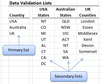
But what if you want a second data validation list to only show values that are specific to the first list, like the one below?
Well, that’s exactly what Jackie emailed me about the other day, and here's how you do it.
How to set up Dependent Data Validation Lists
First of all enter the data for your lists. These are mine:
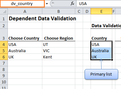
Now, give your primary list a named range.
To insert a Named Range:
- Highlight the range of cells containing your list, excluding the header.
- Up in the name box (the name box is highlighted by the orange box in the image below) type in the name you want to use (with no spaces) and press ENTER. As you can see, mine is called dv_country.
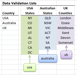
Now give your secondary lists named ranges too.
Here’s the trick: you must use the data from your primary list for your secondary list names.
So, my secondary list for the USA states is called ‘usa’, Australia’s secondary list is called ‘australia’ and the UK list is called ‘uk’ as you can see in the image below.
Now you’re ready to set up your data validation.
Setup Data Validation
- Choose the cells you want validated using your first list. Mine are A4:A6.
- On the Data tab of the ribbon > Data Validation > Data Validation
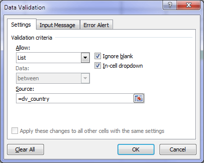
- Choose ‘List’ from the ‘Allow’ field
- Enter the named range for your primary list in the Source field
- Press OK
Setup Dependent Data Validation
- Select the cells you want validated. Mine are B4:B6.
- On the Data tab of the ribbon > Data Validation > Data Validation
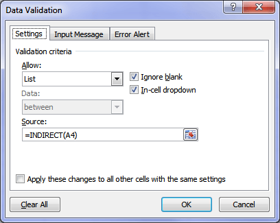
- Choose ‘List’ from the ‘Allow’ field
- In the source field enter an INDIRECT formula that references the first cell containing your primary data validation. Mine is A4 therefore my formula is =INDIRECT(A4)
- Press OK
Bob’s your Uncle (as we used to say when I was about 12).
Enter your email address below to download the sample workbook.
More on Named Ranges.
More on the INDIRECT Function.
Thank you sharing this, I have here a question about same trick: what if I want to select multiple selection! any clue?
Thanks
Mahmoud
Hi Mahmoud,
That is a different problem. By default, it’s impossible to select more than 1 item from a dropdown data validation list. Only with a code this can be done, here is an example for that: selecting-multiple-items-in-data-validation-list
Cheers,
Catalin
Hi Carlo,
Thanks for explaining, it solves some part of my requirement.
Is it possible to have only two columns as a data list say “Country” and “States” in a separate worksheet and under those columns we will have country names repeated in first column and states corresponding to that country in other. How can we use the Data Validation in that case?
For Ex:
A: Countries | B:States
————————
USA | NY
USA | CO
USA | MN
UK | LN
UK | ESS
UK | SOME
Hi Chandregowda,
With your data formatted like that the data validation list will show the countries repeated. The data validation list cannot exclude duplicates. You need to give it a list of unique values first.
So your format will not work for a data validation list. You need to set it up the way it is explained in the tutorial above.
Kind regards,
Mynda.
Hi Mynda,
Is it possible to have several dependents?
I want to use this to specify details.
Here’s the example below.
Primary Secondary Next Then
Country States Village Street
Thankyou.
Hi Jezryl,
Yes. You can! 🙂
Just follow the structure in the example file.
Continuing with our Example, We already have 3 Countries.
If you want to add Villages, then in column C,
add a data validation =INDIRECT(B4) if in row 4, B5 if in 5 etc.
Now, here’s the tedious part. You have to name a range for each state in a country.
For example, You should create name ranges for each of these
states below — and in those ranges should consist of villages.
For example, in ‘NY’ Range you’d have Village1, Village2 etc.
So that when you have NY in B4 and you click the dropdown in
C4, you’ll reference the ‘NY’ named range via B4 thus you’ll
get the list of Village1, Village2 etc.
It’s all about structure.
Cheers.
CarloE
What a great tricks. Thanks a lot.
You’re welcome, Jezryl 🙂
Hi Mynda, I successfully used this example of “Excel Data Validation With Dependent Lists” but there were a couple of things I noticed.
1. In the “Source” box you need to have an “=” Could you change the wording in your example to “=dv_county”.
2. When I entered the “Indirect” function my version of Excel automatically used the absolute value of the cell I selected :-(..so when I copied the equation down the list it still referenced $A$4 .This is a quirk of Excel …. but thought I’d let you know. I love your site. It helps me a lot with curly excel issues and your explanations are very clear.
Hi Rachael,
I’m really sorry for not getting this immediately. I really thought that you’re just making
a comment about the blog post but at second glance it seems you were in fact asking a question.
On number 1, Yes you can change it; provided, you change the named range. You can go to the
Formulas ribbon, Click Name Manager, Look for dv_country and double click, In the name box
change it to dv_county; that is, if it’s what you mean by this one.
Visit: Named Ranges Basics
On number 2, In all versions, Indirect function is referencing a cell/address indirectly; hence, the name: ‘Indirect’.
To explain it better, we define by example what is direct referencing. So, for example, if you’re
in B1 and you want to write a simple formula to get A1’s value you simply write “=A1”.
So this is direct referencing of a cell.
A1- Dog
B1 -Formula: =A1
Result: Dog
On the contrary, If we use “=INDIRECT(A1)”, we are not referencing
A1 but what is the value in A1. For example, If A1 has a text value of “C1”, then what you will get is the
value –indirectly– in C by referencing A1.
A1 – C1
C1 – Dog
B1 -Formula: =INDIRECT(A1)
Result: Dog (coming indirectly from C)
Note: also that the argument of INDIRECT is not a range, but a text string called ref_text. In other words, this is really the essence
of an indirect; that is, it will not change like the usual direct referencing of ranges. It is not a quirk in other words.
Please visit these blogs by Mynda about INDIRECT with other functions.
Cheers.
CarloE