Knowing Excel array formulas will catapult you to ‘Guru Status’ in your office and I'll do my best to make this painless, but you might need to get a brainbooster (a fruit or veg snack given to the 5 year olds at my son's school at 10am each morning when they're starting to lose focus).
Array formulas are ideal for summing or counting cells based on multiple criteria, a bit like SUMIF and SUMIFS, and COUNTIF and COUNTIFS but better, especially if you only have Excel 2003 and don’t have the *IFS functions.
And unlike the SUMIFS and COUNTIFS functions which only allow you to specify AND criteria, with array formulas you can specify OR criteria too.
Using the data in the table as an example the
SUMIFS is limited to this type of criteria: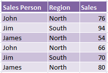
Sum Sales if the salesperson is John AND the region is North
SUMIFS Formula:
=SUMIFS(Sales,Sales_Person,"John", Region,"North")
=142
Whereas with an array formula you can do this:
Sum Sales if the salesperson is John OR Jim AND the region is North OR South
Array Formula:
{=SUM((Sales)*((Sales_Person="John")+(Sales_Person="Jim"))*((Region="North")+(Region="South")))}
=306
We can see from the array formula example above that the * symbol instructs Excel to interpret the criteria as AND, and the + symbol is OR.
Note: the cell ranges in the formulas above have been replaced with named ranges to make it easier to read, quicker to build and easier to follow when you come back to the workbook months later.
Download the workbook and follow along or reverse engineer the formulas.
What is an Array?
An array is a series of data values, as opposed to a single value in one cell. Arrays can be contained in a single row, a column or multiple rows and columns. And array formulas can be entered in a single cell or a range of two or more cells. In this tutorial we’re going to look at single cell array formulas.
You will recognise an array formula in Excel because it is enclosed in curly brackets { } see example above. These curly brackets are inserted by pressing CTRL+SHIFT+ENTER upon entering the formula, and as a result array formulas are sometimes known as ‘CSE formulas’.
Array Formula Example
Let’s take a look at what’s actually happening in Excel when we insert an array formula.
Excel array formulas are testing for TRUE or FALSE outcomes with a numerical equivalent for TRUE being 1, and for FALSE being 0. These TRUE or FALSE values are known as Boolean values.
Taking the above example Excel is finding whether the values in the salesperson column are either John or Jim, and awarding the cell a 1 or a 0 based on the outcome.
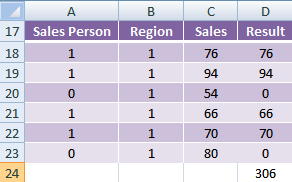
So the Sales Person values are {1,1,0,1,1,0}
It then does the same for the Region:
{1,1,1,1,1,1}
And then multiplies these outcomes by the Sales column and adds up the result for each row:
{1x1x76}+{1x1x94}+{0x1x54}+{1x1x66}+{1x1x70}+{0x1x80} = 306
How to Enter an Array Formula
As mentioned earlier, array formulas are surrounded with curly brackets. You must not type in these curly brackets (if you do your formula won’t work). They must be entered by pressing CTRL+SHIFT+ENTER when you enter the formula, as opposed to just pressing ENTER.
You will notice the curly brackets disappear when you edit the cell. When you’re finished editing you need to press CTRL+SHIFT+ENTER again to enter the formula correctly.
Note: While the SUMPRODUCT function is an array formula it doesn’t require curly brackets, or to be entered using CTRL+SHIFT+ENTER.
Array Formula Examples
Using the sample data on the right let's work 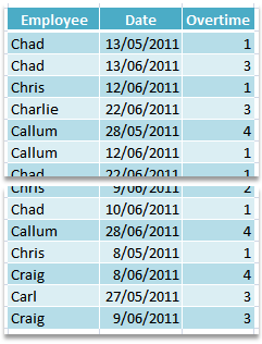
through some scenarios.
Note: Again I've used named ranges for each column (Employee, Date and Overtime) as you will see in the formulas below.
COUNTIF Using an Array Formula and a Date Range
If you have Excel 2007 or Excel 2010 you can do these with the COUNTIFS function.
Scenario 1
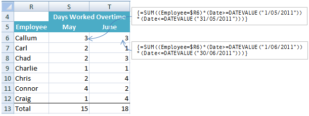
Count the number of overtime days worked per person for each month
Array Formula for May in cell S6
{=SUM((Employee=$R6)*
(Date>=DATEVALUE("1/05/2011"))*(Date<=DATEVALUE("31/05/2011")))}
Array Formula for June in cell T6
{=SUM((Employee=$R6)*
(Date>=DATEVALUE("1/06/2011"))*(Date<=DATEVALUE("30/06/2011")))}
Result
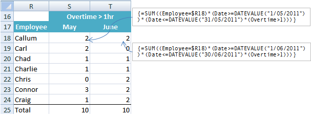
Scenario 2
Count the number of overtime days worked per person each month that were more than 1 hour
Array Formula for May in cell S18
{=SUM((Employee=$R18)*(Date>=DATEVALUE("1/05/2011"))*(Date<=DATEVALUE("31/05/2011")*(Overtime>1)))}
Array Formula for June in cell T18
{=SUM((Employee=$R18)*(Date>=DATEVALUE("1/06/2011"))*(Date<=DATEVALUE("30/06/2011")*(Overtime>1)))}
Result
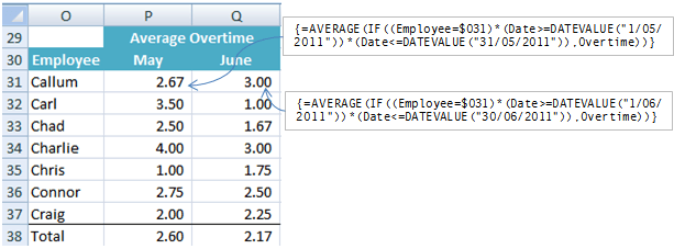
AVERAGE Using Array Formulas
Scenario:
Average the overtime hours worked per person each month
If you have Excel 2007 or Excel 2010 you can do this with the AVERAGEIFS function.
Array formula in cell P30:
{=AVERAGE(IF((Employee=$O31)*(Date>=DATEVALUE("1/05/2011"))*(Date<=DATEVALUE("31/05/2011")),Overtime))}
Result
Note: When the IF function is used in an array formula it evaluates slightly differently. It creates an intermediate array using cell references for TRUE, and ‘FALSE’ values for FALSE.
For example an intermediate array might look like this:
{FALSE, FALSE, FALSE, FALSE, N10, N11}
Where N10 and N11 are TRUE i.e. they match the criteria. And since the average function in Excel is set to ignore Boolean values it will only average N10 and N11 ignoring the FALSE values thus creating a true AVERAGE.
Array Formula Rules
1. The ranges referred to in your array formulas must be the same size, otherwise you will get an error. For example in the formula below you can see that although the formula may refer to different columns of data the length of the column is from row 6 to row 11 in each case.
{=SUM((C6:C11)*((A6:A11="John")+(A6:A11="Jim"))*((B6:B11="North")+(B6:B11="South")))}
2. To enter the array formula you must press CTRL+SHIFT+ENTER, that is hold down CTRL and SHIFT and then press ENTER releasing all of them together. If you use a Mac it's COMMAND+RETURN.
3. Do not enter the curly brackets yourself, Excel does it when you press CTRL+SHIFT+ENTER.
4. When the multiplication symbol * is used it means AND, and when the plus symbol + is used it means OR.
Enter your email address below to download the sample workbook.

I believe there is a typo within the formulas in the Scenario 2 paragraph? I am copying below:
Array Formula for May in cell S18
{=SUM((Employee=$R18)*(Date=DATEVALUE(“31/05/2011”)*(Overtime>1)))}
Array Formula for June in cell T18
{=SUM((Employee=$R18)*(Date=DATEVALUE(“30/06/2011”)*(Overtime>1)))}
If you compare this with the result embedded image you can see that you have mistakenly used =DATEVALUE(“31/05/2011”), whilst it should be the other way round? Am I correct?
Good catch, Yiannis. Thanks for letting me know. Fixed now.
Very cool stuff! I had some problems with CTRL SHIFT ENTER. When you copy and past the formula into a cell you gotta place cursor at the end and then press CTRL SHIFT ENTER.
Thank you for your detailed explanation!
Hi Igor,
Glad you liked it. Good point about pasting. If you copy the cell and paste it you don’t need to press CTRL+SHIFT+ENTER, only if you edit the cell before copying the contents of the cell and then paste that, will you have to enter it with CTRL+SHIFT+ENTER.
Mynda
Thank you again, Mynda!
Hi Mynda,
Could you please confirm whether the array formula also work in Excel 2013? And if so, any difference?
Plus, the workbook used is a bit out of date with the cell reference quoted in the post.
Cheers,
Frank
Hi Frank,
Yes, these array formulas will also work in Excel 2013 but if you can use the built in functions like SUMIF/SUMIFS or COUNTIF/COUNTIFS then always choose them before an array formula.
Thanks for letting me know about the cell references. I’ve updated the file.
Cheers,
Mynda
Hi Mynda,
Just wondering would I be able to use the sumifs function in cell S18? The difficulty with Array formula is that I can get guidance from the “insert function”.
The syntax I used is =SUMIFS(Overtime,Employee,$R$18,Date,>=datevalue(“1/05/2011”),Date,<=datevalue("30/05/2011"))
and it doesn't seem to work.
Cheers,
Frank
Hi Frank,
Yes you can but you have to make some modifications to the >= criteria like so:
=SUMIFS(Overtime,Employee,$R$18,Date,">="&DATEVALUE("1/05/2011"),Date,"<="&DATEVALUE("30/05/2011"))I write about this here: https://www.myonlinetraininghub.com/sumifs-formula-referencing-cells-containing-dates
Kind regards,
Mynda
Hi ! I was looking for a formula which helps in the following scenario :
I got 5 sheets in a single work book- sheet 5 (master sheet) has to be compulsorily updated- other 4 sheets has to be updated with bits-n-pieces data 4m sheet 5. Is it possible 2 derive a formula that would help
Hi Sumiit,
Can you please upload a sample of your workbook, with detailed descriptions of what you want to do? You can use our Help Desk: https://www.myonlinetraininghub.com/helpdesk/
Catalin
Dear Mrs. Linda,
I was trying to download examples by clicking “Download the workbook”, but when I unzip file, there is only a folder structure with many xml files, so I can’t find any workbook to open it with excel.
Please, advice me, how to do it, or make me know where do you have a reference page with explanation (if exists).
Thank you in advance,
Lado
Hi Lado,
That’s because it’s not a .zip file. Your browser is changing the file extension on download. If you hover your mouse over the download link you can see that it’s actually a .xlsx file.
What you need to do is download it again but this time type over the .zip file extension with .xlsx at the ‘save as’ screen (or equivalent for your browser) and then when it has downloaded you can open it like any other Excel file.
Let me know if you have any problems.
Kind regards,
Mynda.
Hi,
I tried to download the workbook, but all files are xml, not excel.
Hi Peter,
The workbook is a .xlsx file. Try renaming it or download it again and make sure your browser doesn’t change the file extension. You can type over it with .xlsx in the ‘save as’ window.
Kind regards,
Mynda.
Hi Mynda,
How can I use array into RANK function?
In your example, I want calculate rank of sales person from its regions. I calculate all sales for each region and I calculate the percent for the sales person. For each sales person I have a percent of sales for his region. Now I want calculate rank of each sales person.
The RANK function is: RANK(sales percent of person, all percent of his region). How do I do this dynamics? (Dynamic second argument of function.)
My idea is simply but don’t work. I calculate in column D percent of each sales person from his region. Total of region is simply to calculate (sumif or sumproduct). I sort by region to have successive region. Now I have first of argument for RANK function and for second argument I try something like ($D$6:$D$11)*–($B$6:$B$11=B6). This return an array but I can’t use for second argument in RANK formula.
Any idea? Any suggestion?
Thank you.
Best regards,
Sorin.
Hi Sorin,
Have you read this post on different ways you can RANK data?
If that’s not what you need can you please send me your workbook via the help desk so I can see what you’re working with.
Thanks,
Mynda.
Hi Mynda,
Your post with RANK is all I need! 🙂 I made some change and it’s work.
I didn’t saw the post before ask the question.
Thank you very much.
Best regards,
Sorin.
Great 🙂 Glad it helped.
I would like to get a multiplication value as per the following
c1 having value (10) in sheet1 * c1 (20) in sheet2, if a1(“pet”) in sheet1 matches with a1(“Pet”) in sheet2 and give the result in d1 in sheet1.
Kindly help me with the formula.
Vincent
Hi Vincent,
I think this is what you mean:
Kind regards,
Mynda.
Reply to myself 😉
So, with your formulas, I had to change the month-day order in the dates. And I had to tell it what I was summing — ie: I added (Overtime)* to make it {=SUM((Overtime)*(Employee=$O7)*(Date>=DATEVALUE(“6/1/2011”))*(Date<=DATEVALUE("6/30/2011")))}
It appears the formula doesn't work if any cell in the range to be summed is text. Unfortunate since SUMIFS works, but does not allow for OR criteria.
Any ideas?
Hi Meggan,
;( 🙂
Wooohkay… Honestly I don’t exactly know the answer. lol.
However, If you need some crazy idea, It’s like this…
SUMIF and SUM are all functions built some genius in the creators of Excel
–no sarcasm there. They have tried to the best of their abilities
to anticipate the anything-goes needs for people like us.
SUMIF therefore was built to be very specific –hence no problem– while SUM/SUMPRODUCT
are nice attempts of a do-it-all-almost functions. You can’t argue with SUMIF
because it requires very specific arguments no if’s and no but’s. On the other hand,
SUM allows complications particularly in an Array Formula. So perhaps the one who made the SUM function
got tired of anticipating possible errors like adding a text and a number.
He could have troubleshoot it but he decided : SUM are for numbers and not text. lol.
Seriously, Some functions are so great in anticipating this while some are not.
If you notice, the more difficult the task for a function is the more it is stricter as to its
arguments. For example, SUM not in an array. It would have a logic like this:
Loop each cells highlighted
(if cell value is not a number change to ZERO)
cell + cell
result: SUM of Cells
You see in programming(as Excel is an application, a program), Data types should be consistent
especially numeric ones. You need logic or error handlers to avoid errors when you will be adding
a text/string i.e. with a numeric one. It might look so simple on the surface but behind it are people
who tried their best to anticipate and avoid these errors.
Think of a very difficult task and maybe you’ll consider the creators of Excel to be human afterall. 😉
Moral Lesson: Please do not ask the “why” of the matter. 😉
Send your concern regarding the “how” and its possible workaround here HELP DESK.
Cheers,
CarloE
Thanks for your reply, Carlo. =) If I had paid attention to the “Average” bit and to using an intermediate array, I wouldn’t have bothered you. Another good lesson for me, hahaha. Forcing that array lets me use text values in a column to be summed because they get dropped earlier than the SUM.
This site has been super helpful; thanks for keeping it up!
Hi Meggan,
You’re welcome.
Cheers,
CarloE
Hi, I was excited to use these in a project. However, I can’t make it work — I always get #VALUE errors, even in the workbook I downloaded from this site.
When I first downloaded and opened it, all the numbers in ‘Array Formulas’ O5:Q14 were there. I clicked in the formula, changed nothing, then used Ctrl+Shift+Enter to exit the formula; it resulted in the error. The curly brackets get added, but no values. =(
Whaaa? Office Pro Plus 2010 on Win 7 Ent 7 SP1
Ok, I know this answer is way too late, but I just picked up this lesson tonight, found it very useful, and encountered the same error that Meggan did. I figured out my copy of the spread sheet was having trouble with the date value. I am using 2013. I put the dates, May 1, 2011 in cell U6 and May 31, 2011 in cell V6 first, then I made the formula refer to those cells for the dates rather than using the Datevalue and a text entry of “1/5/2011”. This seemed to clear up the error.
this is the formula i have now: {=SUM((Employee=$R6)*(Date>=$U$6)*(Date<=$V$6))}
hope this helps anyone who happens upon this lesson after me.
I’ve been looking for a way to concatenate/append arrays. I have used many programming languages with array capability that allow for concatenating/appending arrays.
I have two arrays (as rages, or named arrays), and I want to be able to concatenate/append them into a single array for other manipulations. However, I have yet to find an Excel function/operator/whatever that provides for this functionality.
In my present case, I have the simple situation of two one dimensional vertical arrays, and I want a single one dimensional vertical array formed from the elements of the first array followed by the elements of the second array.
Is there a built-in function/operator/whatever to do this? (I know I could do it in Visual Basic, but I suspect that may slow my spreadsheet down even more than it already is.)
Hi David,
Try this formula.
Note: first is a named range (single column)
jam is a named array horizontal (={“jay”,”wash”,”olsen”})
jom is a named array vertical (={“jay”;”wash”;”olsen”})
RESULTS:
*b is first and jam
*c is first and jom
similar results.
The ROW function simply is an INDEX to the range and arrays respectively. So if you notice when you will
try this experiment, the Row will increment from A1 to A2 etc. which will return values 1,2 etc. thus
pointing to the right range/array row.
Read more also on : Named Range, Index, Iferror
Cheers.
CarloE
Hi Mynda,
Just on question ( i know i will sound stupid after this), in above Countif example you have used named range as DATE. we have also a DATE formula in excel… will that cause any problem.
Is it a good practice to avoid using names of excel formulas ?
Hi Pradeep,
You’re right using them isn’t a good practice.
But if excel allows it, then it’s not totally
a ‘bad’ practice’. One bad thing about
this one is that it does create a little confusion
when a user relies on the autocomplete feature of a formula
because two ‘Dates’ will appear, the named range and
the function Date. Even then, It’s not a big issue because
in the final analysis the two can be distinguished. The
function shows a screen tip (i.e. its arguments) while a
named range doesn’t.
Regarding VBA code, a named range is invoked with the use
of double quotes (“”) very much like a string. So there’s
no problem with that.
So it’s up to the user whether to obey good practice or
use meaningful names like ‘DATE’ for ones consumption.
Most importantly, Excel stops the user from pursuing things
which it really does not allow.
See rules in naming a range.
Cheers.
CarloE
Hi Mynda,
I’m arriving a bit late to the party, but thought I’d offer an alternative to using the DATEVALUE formula. Instead I used TEXT(Date,”mmmm”) where Date is the named range. I set this equal to the cell with the month value. So the equivalent formula for:
‘{=SUM((Employee=$R6)*
(Date>=DATEVALUE(“1/06/2011″))*(Date<=DATEVALUE("30/06/2011")))}
is:
={SUM((Employee=$R6)*(TEXT(Date,"mmmm")=S$5))}
Not sure if there are any disadvantages for this approach, but it works for me. I enjoyed the article – thanks for posting.
Hi Martin,
Love it! I might share that in a future blog post 🙂
Cheers,
Mynda.
Hi Mynda,
Should I use an array formula to return multiple vlookup results?
See below ex. Say I want to retrieve each shop for article 1 in a separate column. I can use vlookup but it only returns the 1st found value. How do I retrieve the 2 shop names in 1 separate column? Is an array formula the solution?
Article 1 Shop1
Article 2 Shop2
Article 1 Shop2
Article 4 Shop3
I hope you can help me. Thanks in advance.
Karine
Hi Karine,
Yes, you can use an array formula to lookup and return multiple values. Here is a tutorial on this exact topic.
Kind regards,
Mynda.
When I download your sample spreadsheets from the link above in ZIP format all I get are a lot of XLM files. What am I doing incorrecly?
Hi Dwight,
The problem you are having is your browser is changing the file extension to a .zip file when you download it. If you hover your mouse over the link and look in the bottom right/left of your browser you will see the correct file extension is a .xlsx
You need to download the file again and at the ‘save as’ screen (or equivalent for your browser) type over the .zip file extension with .xlsx
You will then be able to open the file in Excel as normal.
Kind regards,
Mynda.
Hello Mynda
Now that I’ve been able to look at the full dataset, my query is resolved.
The results reflect the number of entries in the list, rather than the overtime hours worked. Sorry to be a pest!
Thanks and regards
Hercules
Hello
I suppose it must be me, but I couldn’t understand how you got the results for cells S6 and T6 from the sample data in the first example.
The sample data doesn’t have any row/column refs, so I thought Id download the workbook and look at that. But… I couldn’t find any reference to the S6/T6 example in what was downloaded from the link.
Also.. If I clicked on any of the tutorial links Excel (2010) told me that the operation was cancelled. As I am unable to view any of your examples in full, Im afraid that it isn’t any help to me!
Hi Paul,
Sorry you’re having trouble. If the links in the downloaded workbook aren’t working it’s usually because you haven’t enabled the workbook. When you download a workbook Excel disables it for your protection. There should be a yellow band above the formula bar with a notification asking you to ‘Enable Workbook’. You need to click this before the links will work.
In the tutorial above there are no row or column references in the sample data because I have given them named ranges. You don’t need to know the references, just the named ranges.
I hope that helps.
Kind regards,
Mynda.
Hi Mynda,
Very neat and clean explanation of how an Array works. I have browsed many websites but yours is certainly at the top.
Thanks.
Regards,
Vivek Sahasrabuddhey
India
Cheers, Vivek. It’s rewarding to know I’ve been able to help 🙂
I trying to create formula in excel that text & numbers in next column having in each rows, but in between I don’t want one of the word or text & number of particular row.
How to create a formula. Please help writing formula. Email to my ID which is mentioned. Below columns & rows.
Sl.No. Items ABC XYZ PQR
1 Pen 10 8
2 pencil 12 4 8
3 chocalate 24 18
4 cream 8 6
5 eraser 12 6 20
Hi Kumar,
I’m having difficulty understanding what you want. Can you please give me an example of the end result so I can see how to get from A to B and give you a solution.
Kind regards,
Mynda.
Please provide me the details of all array formulas.
Thanks
Chandra
Hi Chandra,
If only it was that simple. There is no limit to the combinations of array formulas (well, statisticians would say there is a limit but it would be a ridiculously large number), so it really is a case of understanding how they work and then playing around with combinations of nested functions to get your desired results.
I’m sorry I can’t give you an ‘array formula bible’ 🙁
Kind regards,
Mynda.
I have an array formula created. I don’t know how it got there, but it’s there now. When I try to do something as simple as change the value of a constant, I receive a #VALUE error.
This is what I have entered in the cell:
=B15+1.96*MMULT(MMULT(TRANSPOSE(H9:H11),B4:D6),H9:H11)^0.5
Changing ANYTHING, even 1.96 to 1.95, returns the #VALUE error.
Please advise.
Hi Harlan,
I can’t tell without seeing the workbook. You can send it to me via the Help Desk and I’ll take a look.
Kind regards,
Mynda.
Hi! Could you tell how to use the Vlookup function with Arrays.
Further, i have been using the IF + ISERROR + VLOOKUP with COLUMNS Function extensively. Generally these files are of sized 5MB to 10MB size. However, when ever I run this formula, i find that, my system takes lot of time, some times it hangs up (not responding). Could you suggest, any better way?
Thanks & regards
Raghu A J M
Hyderabad, India.
Hi Raghu,
There are (almost) endless ways to use a VLOOKUP in an array so I’d need an example of what you want to achieve before I can answer your question.
Your IF + ISERROR + VLOOKUP + COLUMNS function is probably slow because (I suspect) you are requiring Excel to do the calculation twice. Once to find if the result is an error and a second time to find the result if it’s not. e.g. =IF(ISERROR(VLOOKUP(A1,$E$1:$G$100,3,FALSE)),””,VLOOKUP(A1,$E$1:$G$100,3,FALSE))
You can try to use Database Functions where appropriate as an alternative.
It’s not a good idea to use ISNA, or ISERROR in your case, with a VLOOKUP.
I hope that helps.
Kind regards,
Mynda.
The website very herlpfull to beginners
Cheers, Scott.
Thanks for the materials you have been offering. It keeps me updated with various tools of excel!
THIS is THE BEST, MOST straightforward explanation on array formulas that I’ve seen on the web…THANK YOU for publishing it and demystifying it!!!
🙂 Thanks again, Scott.
I think Array formulas are quite a scary concept for loads of people (me included), but once you understand the logic and practice them a bit, you can start to think in terms of arrays, and they become a powerful weapon in your Excel arsenal.
Cheers,
Mynda.