Navigating workbooks with lots of sheets can be tedious. In this tutorial I’m going to show you how to dynamically list Excel sheet names and add some user-friendly hyperlinks to help users easily navigate the file.
It requires an old Excel 4.0 Macro Function called GET.WORKBOOK and this means the file must be saved as a .xlsm file type. Don’t let that put you off though. It’s super easy and doesn’t require any macro/VBA programming knowledge.
Watch the Video

Download Workbook
Enter your email address below to download the sample workbook.
Formula to Dynamically List Excel Sheet Names
The crux of this solution is the GET.WORKBOOK function which returns information about the Excel file. The syntax is:
=GET.WORKBOOK(type_num, name_text)
type_num refers to various properties in the workbook. Type_num 1 returns the list of sheet names and that’s what we’ll be using.
name_text is the name of the workbook you want to get the sheet names from. We’re going to omit this argument, and it will simply return the names from the active workbook.
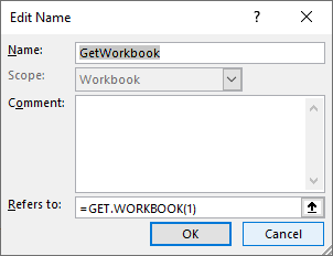
Excel 4.0 macro functions like GET.WORKBOOK cannot be typed in cells like the functions we know and love today, they must be defined in a name.
I’ve defined a name (Formulas tab > Define Name) GetWorkbook as you can see below:
And if I reference that name in a formula it returns the list of sheet names prefixed by the file name.
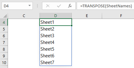
You can see in the image below that I wrapped the defined name in the TRANSPOSE function because GET.WORKBOOK returns a horizontal array of sheet names and I wanted them in a vertical array.
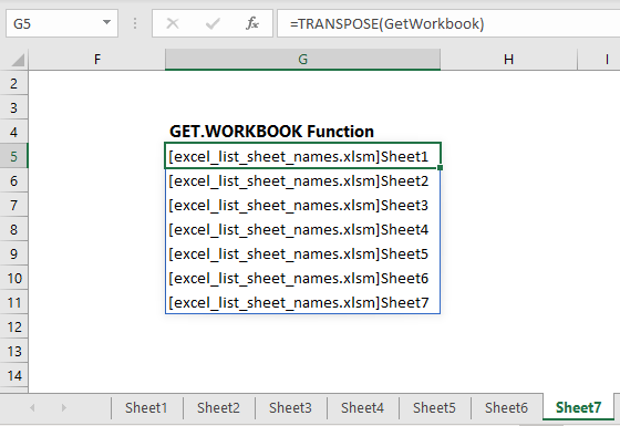
Note: I have Excel for Microsoft 365 with dynamic arrays, so my formula spills the results to the cells below, as denoted by the blue border around cells B6:B12 in the image above.
If you have Excel 2019 or earlier you need a different formula, but more on that later. First, I just want to explain what GET.WORKBOOK does.
Now, I only want the sheet names, so I’ll use the REPLACE function with FIND to extract them:
=REPLACE(GET.WORKBOOK(1),1,FIND("]",GET.WORKBOOK(1)),"")
Tip: you could use the SUBSTITUTE function instead of REPLACE.
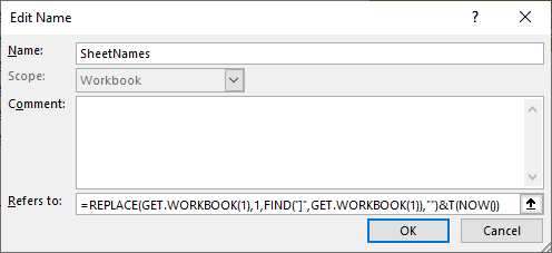
Lastly, to ensure the formula dynamically updates I’m going to append the volatile function, NOW, wrapped in the T function on the end:
=REPLACE(GET.WORKBOOK(1),1,FIND("]",GET.WORKBOOK(1)),"")&T(NOW())
We do this because NOW, which returns the current time, triggers a recalculation of the defined name. The T function returns blank when the value returned isn’t text. In other words, T hides the time returned by NOW. The only reason we’re appending the NOW function is because it’s a volatile function that triggers a recalculation of the defined name which is required to update the list of sheet names.
I’ll define a new name for this formula, SheetNames:
And when you enter this formula wrapped in TRANSPOSE in a cell it returns the sheet names:
Again, my formula spills the results to the cells below because I have dynamic arrays.
Dynamically List Excel Sheet Names - Excel 2019 and Earlier
In all versions of Excel we can use the INDEX function with ROW to return the list of sheet names:
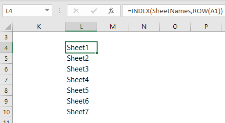
Note: the ROW function simply returns the row number of a cell. The ROW function in the formula in the image above returns 1. As you copy it down the column it returns 2, then 3 and so on. However, if you copy the formula down more rows than you have sheets for it will return an error.
We can handle the errors with the IFERROR function:
=IFERROR(INDEX(SheetNames,ROW(A1)),"")
This allows you to copy it down past the current number of sheets you have which will ensure any new sheets added are automatically included in the list.
Dynamically List Excel Sheet Names with Hyperlinks
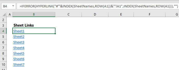
Of course, what good is a list of Excel sheet names without hyperlinks to take you to those sheets? To solve this we can nest the INDEX formula inside HYPERLINK:
=IFERROR(HYPERLINK("#'"&INDEX(SheetNames, ROW(A1))&"'!A1", INDEX(SheetNames,ROW(A1))),"")
Copy the formula down to get a list of sheet names with ready-made hyperlinks:
Be sure to copy the formula down past the last current sheet name so that new sheets are automatically included.
More on the HYPERLINK function here.
Note: you may find that the formula doesn’t automatically update. If that happens, press F9 to force a recalculation, or perform any of the other actions that trigger recalculations.
Excel for Microsoft 365
If you have dynamic arrays you might be wondering if this can be done using spilled ranges and the answer is kind of. It requires the sheet name and hyperlink to be in separate columns, as you can see below:
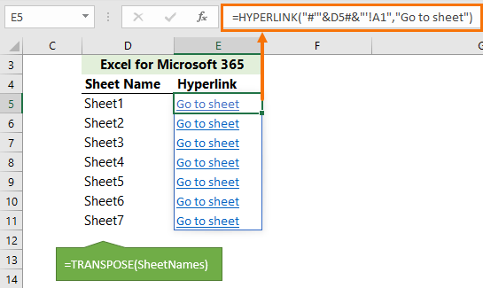
The formula in column D spills the results and will grow as new sheets are added. The formula in column E references the spilled range with D5# and will therefore also grow as new sheets are added. Unfortunately, you cannot create a single formula by replacing D5# in column E’s formula with ‘SheetNames’ or ‘TRANSPOSE(SheetNames)’.
Limitations
This technique has a few limitations:
- It includes hidden sheets however the hyperlink can't open a hidden sheet
- It requires the file to be saved as a .xlsm and macros enabled
- Requires recalculation to add new sheets to the list. The T(NOW()) part of the formula will trigger recalculation based on various actions, but if you don’t perform any of those actions, you can force a recalculation by pressing the F9 key.
Related Lessons
We can also generate a list if Excel Sheet Names with VBA
And you can get a complete list of the elusive Excel 4.0 Macro Functions here.

Hello Minda, your explanation is flawless and initially i was able to get the desired output but once i saved the file as .xlsm and closing and reopening the list disappears.
tha defined name and formula are properly saved but the return data shows as blank cell.
Even on pressing F9 the data cell returns as blank.
What can de done to resolve this error?
thank you for the write up and all the help you provide.
Regards
Hi Ritesh,
If your files are saved on OneDrive and the file path is a URL, then FILES will not be able to extract the file names. Could this be the issue?
Mynda
No. The Workbook in in thr Local HD.
I worked the same file on a separate Laptop on which MS Office Professional 2016 is installed and it worked as intended.
Again i tried on the first Laptop but the result remains the same as per the original query. on this laptop MS Office HS 2021 version is installed. I am not sure if the different versions has to do anything with the formula.
i think it has something to do with Macros?
any particular macro setting that you can think of may be causing this behaviour?
Regards
Yes. Follow the Macro settings here.
Hi Mynda,
I am also experiencing this problem with the disappearing list. The file is saved on OneDrive/SharePoint. Do you know how to work around this issue so I can utilize the dynamic hyperlinked list?
Hi Cindy,
The issue is likely due to the fact that the formula only works while the workbook is open and macros are enabled so the formula can be recalculated.
When the file is reopened, the defined name referencing `GET.WORKBOOK` may not automatically refresh or may return a blank if:
– Macros are disabled
– Calculation hasn’t been triggered
– The workbook opens in Protected View
If any of the above don’t happen, the name is used in the formula INDEX(SheetNames,ROW(A1)) ends up referencing an empty or null array on open.
One solution is to trigger a recalculation:
Make sure the workbook is set to ‘automatic calculation’ (Formulas tab) and that `NOW()` or some other volatile function triggers a recalc:
– Add a helper cell like `=NOW()` somewhere to force updates.
– Ensure users click Enable Macros when prompted.
Mynda
I was wondering if there was a way to limit the list of worksheets output by the Get.WorkSheet macro function. I have say X number of sheets but only want to start listing from worksheet #3. Can that be done?
Hi Matthew,
Yes, you can wrap the TRANSPOSE(GetWorkbook) formula in any function that filters a list, like FILTER, INDEX, TAKE, DROP etc. For example, with the formula below you can return rows 2, 3 and 4:
=INDEX(TRANSPOSE(GetWorkbook),{2;3;4})Mynda
This is AMAZING!! THANK YOU!
You’re welcome. Glad it was helpful
I have two columns; one is for sheet name and the other for tracking some activity. If I delete the sheet from the workbook, I need the entire row to be deleted, and when I add a new sheet a new blank row should be created. Any tip for this.
Thanks for the support.
Hi Prashant,
Pressing F9 will recalculate the formulas to include any new sheets, and any deleted sheets are automatically removed from the list. Unfortunately, this will result in any data you’ve added in adjacent columns to be out of sync with the list of sheets. I don’t see any easy way to have both a dynamic list of sheets and have the data you’ve stored in adjacent columns to stay in sync using this formula approach to listing the sheet names. You might need to write a VBA routine to handle this instead of this formula approach.
Mynda
TYPO Alert:
Excel LET Function allows you to declare variables and intermediate cacluations
cacluations
what’s my reward?
Your reward is our thanks!
Dear Mynda,
Is there a way that I can exclude the first sheet (Tutorial) from the list of sheet names displayed as Hyperlinks in the 2nd method (Dynamic Arrays)? I was able to do it in the Index formula method wherein I started from Row(A2) instead of Row(A1).
Thanks,
Rajiv
Sounds like you answered your own question, Rajiv. If you’re still stuck please post your question on our Excel forum where you can also upload a sample file and we can help you further.
This was fantastic!! Thank you so much. The video was very well done, and the transcribed text helped me get the formulas just right. Good timesaver and will be returning here for future questions! Thank you,
Great to hear, Dave!
Love this post, informative and adding the T(NOW()) solved a huge problem I was having!
Great to hear!
There’s always some hidden tip within a tip, and this time it was the use of T(NOW()) to make the function volatile. I have used “+ N(“some text”)” to document functions in a similar but opposite manner.
Great to hear you found some nuggets in this post
Great to hear you found some nuggets in this post, Patrick
Great to hear you found some nuggets in this post, Patrick
Hi there thanks for the great solution!
Oddly, when I close the excel sheet and open again, my sheet name column would return #N/A. I have to manually go to define names and click the saved SheetNames again.
How do I ensure that excel automatically uses SheetNames when it starts up?
I’m not sure what would be causing this. Please post your question on our Excel forum where you can also upload your file and we can help you further.
Hello and thank you for this video. It has helped me merge two different reports into one data source.
I am coming across something when I add some data to the existing two spreadsheets and then press the Data/Refresh All button.
The query data is added as additional data into the combined data sheet so it is doubling the information. How do I prevent this from happening?
Hi Rob, I think you meant to post this comment on this post https://www.myonlinetraininghub.com/power-query-consolidate-excel-sheets. You need to filter out the query table from the ‘source’ data as it’s including this sheet/table in the query because you’re getting all sheets/tables in the current file.
Hi Mynda! Thank you for the tip about listing a number of sheets. Years ago (2015-2017) I worked on a technical project about Intelligent Signaling Systems (ITS) on a highway.
My designed sheets was both design, semi automated Quality assessment and always the latest “final” blueprint. I had of 195 sheets in one workbook with each sheet prepared to be printed out as a A4 paper (a size used in Northern Europe close to Legal size). My sheets should make sense if printed out as you can imagine.
On each sheet I had the name of the sheet (so it could been seen on a printout and you could refer back to Excel workbook sheet at a later day). I used the following dynamic text-formula:
MIDT(@CELLE(“filnavn”;P104);FIND(“]”;@CELLE(“filnavn”;P104))+1;255)
I am using a Danish translation of Excel, so sorry for the commands. Line 104 happened to be the title line on the printout.
Due to the many sheets, it had to be short, uniq and descriptive, so I could navigate among the sheets, but as support for future users I had to add a sub title on each sheet which I referred to on the index page.
On the indexpage I had the page number on the printout, Excel sheetname, descriptive subtitle, revision date (each sheet had individual revision date to make it easier to find latest revisions for the external PLC programmer).
I used a method similar to your video blog on the index page, except of the extra columns, so I don’t need to write it here.
Hi Marie Louise,
Thanks for sharing your interesting story. I dread every having to work in a file with that many sheets 🙂
I did wonder why you didn’t use the header/footer print options to automatically insert the file &[File] and sheet names &[Tab] when printing. I’m sure you had your reasons, but I thought I’d mention it here for those who may read these comments in future.
Mynda
Hi Mynda
I will use that option today, but I had a frame around all data that needed printout and would avoid holes between header and footer (in the frame). The authorities couldn’t decide on some of the signalling along the 3 mile long project area, so I had to add and remove on short notice. I used the group function to add/remove data from printout should they wish. Actually I can’t remember why.
Each sheet had 104 row and 20 coulumns. The last 12 coulomns was a design of 12 different timers (The cells showed what signalimage a future driver would see), but in most cases I could do it with up to 6 timers. That gives an enormous amount of data to keep track of. A “wrong” signal could confuse a driver and result in a traffic crash.
The page number had a break between 7 and 10 and again after page 97. I had to nummerate the pages myself in this case.
A fun side effect of all my efforts was an external consultant added macros to test my design so we could see how cars would “see” my signaling in almost real time in the 16 different traffic options. I had the pleasure to correcting a few errors in the macroes without knowing anything about VBA, but due to the many sheets and data we had to replace the formulas with the displayed text. We did that by adding the value on top the formula cells. Otherwise the macros would either run very slowly at best, or not at all.
That led to macro courses online 😀
Marie Louise
I knew you’d have a good reason 🙂 Sounds like a very rewarding project!