In this tutorial we’re going to look at how we can create a single Excel Slicer for Year and Month, as opposed to the default of having the Year and Month in separate Slicers.
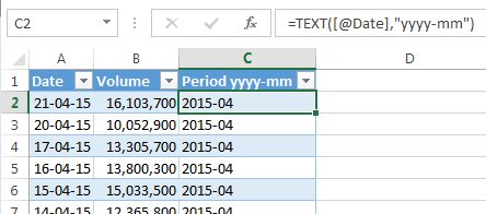
Let’s rewind a tad and look at how we got here in the first place. Below is an extract of my data; it’s a list of trading volumes spanning 13 months from April 2014 to April 2015.
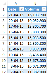
Note: my dates are dd-mm-yy.
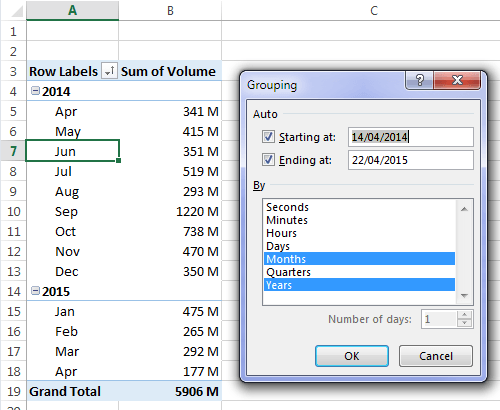
When I created the PivotTable I grouped my dates by Years and Months (right-click > Group):
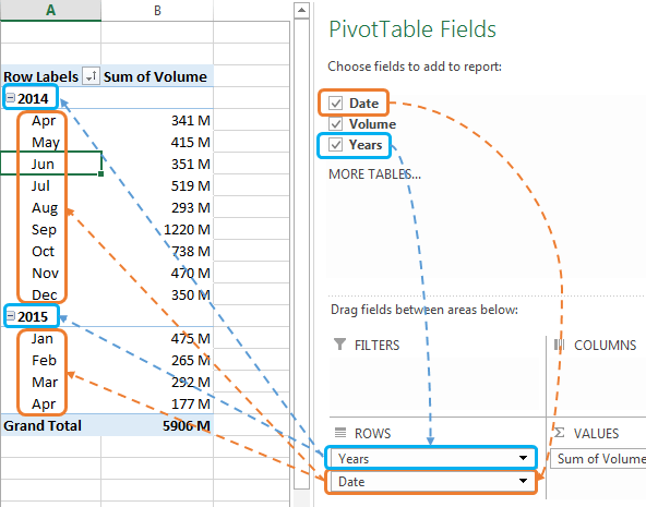
This adds a new field to the Field list for the Years and the Date column now displays the Months in the PivotTable:
Download the Workbook
Enter your email address below to download the sample workbook.

Watch the Video

Slicers for Years and Months
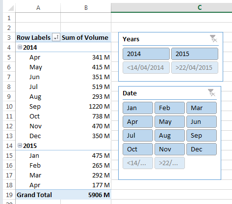
Here’s the rule, you can only have one field per Slicer. In other words, you can’t combine fields from the Field List into one Slicer. So as it stands if we wanted to add Slicers for Years and Months then we could, but it would look like this with two separate Slicers:
You might have noticed there are two things that aren’t ideal with the one Slicer per field method:
- The Years are separate to the Months which means the user has to click two Slicers to select the period they want and if they’re not careful and only select the month, for example April, they’ll get April values for 2014 and 2015 added together, and it’s highly unlikely they’ll actually want that.
- You might have noticed the Less Than and Greater Than buttons in the Slicer. They are automatically inserted when you group your dates, and there is no way to remove them. The best you can do is make the Slicer smaller so you can’t see them, but then you have a scroll bar in the Slicer (see below) and you know some nosey parker is going to scroll down and then get confused:

The Solution
Since Excel won’t allow you to combine fields into one Slicer the solution is to DIY in the source data. It’s easy enough; just add a new column (C) and insert a formula that only displays the Year-Month from the date column:
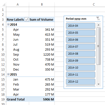
Now you can refresh your PivotTable and go ahead and add a Slicer for the new Field (tip: you don't have to put that field in your PivotTable, you can use it just for the Slicer):
Things to note:
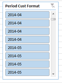 The formula is a TEXT function that converts the date into text and formats it as yyyy-mm. If you just formatted the date as yyyy-mm with a custom number format (as opposed to converting it to text as well), then the PivotTable will ignore the formatting for the purpose of the Slicer and simply display a button for every unique data in the source data (but formatted as yyyy-mm so you can’t see the dd portion of the date):
- I intentionally put the year then the month number, as opposed to month name, or month then year, so that the Slicer sorted the dates in numerical order (even though it’s text). If you format the date as yyyy-mmm e.g. 2015-Apr then the Slicer will have the dates sorted alphabetically like this:
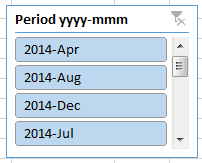
If you prefer your dates like this then the solution to sorting them correctly is to use a Custom List to fix the sort order.
Timelines (new in Excel 2013)
Now, if you’ve got Excel 2013 you might be thinking there’s another alternative, and you’d be right, kind of (I’ll rant about them in a moment). Timelines are a new type of Slicer in Excel 2013 specifically for dates.
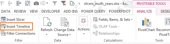
You’ll find them on the Insert tab beside the Slicer button, or in the contextual PivotTable Tools: Analyze tab:
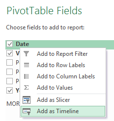
Or if you right click a date field in the Field List:
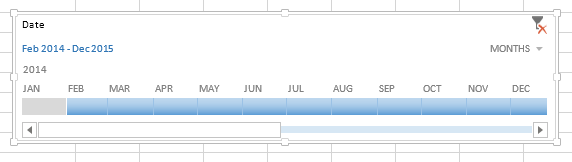
Timelines enable you to toggle between Years, Quarters, Months or Days:
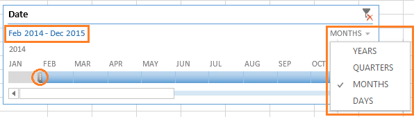
They have a nice scroll bar and clicky-draggy thingy (technical term) to select which periods you want and it even tells you which periods you’ve selected.
And if your data spans entire years they’re almost brilliant, but… I have a list in order of annoyance:
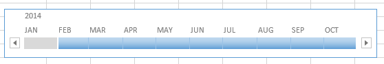
- They’re stupid. I mean they lack intelligence to only present dates that are actually in your data. My data spans April 2014 to April 2015 but the Timeline shows me Jan 2014 to Dec 2015 and it lets me select those dates and end up with an empty PivotTable:
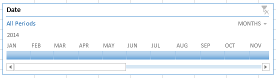
- In their default format they take up 7 rows! Sure you can turn off the header, scrollbar, time level and selection label and they trim down to 3.5 rows, but with that you lose functionality like the ability to toggle between Years, Quarters etc.:
- Like Slicers, you can format them to make the font smaller etc. but (unbelievably) this makes a miniscule difference to their height! Here’s one with 8pt font and it’s still the best part of 7 rows high and if I try to make it any smaller it just cuts off the scroll bar/header:
- In their default format they take up 7 rows! Sure you can turn off the header, scrollbar, time level and selection label and they trim down to 3.5 rows, but with that you lose functionality like the ability to toggle between Years, Quarters etc.:
For those reasons alone I can only see them being useful if your data spans whole years and you have plenty of room for these spreadsheet real estate hogs. Fingers crossed they’re better in Excel 2016.
For now let's stick with Slicers until Timelines are given some more intelligence and formatting flexibility.
Related Topics
- Inserting and using Slicers
- Sorting Excel Date Slicers
- Slicers for Excel Tables (Excel 2013 onwards)
I am glad it is helpful
Excellent needed this quick refence
Glad it will be helpful 🙂
Hello,
I took your advice and created a yyyy-mm Slicer but now that I have created a dashboard that spans in years beginning with 1/1/2020; what about in 2021 when I want to select 1.5 or 2 years of data, so you recommend also adding a “Year” Slicer in addition to the yyyy-mm so that the 2 years won’t need to be selected by dragging all of them? (Also, adding a quarters slicer). I don’t like repeating the year twice but not sure if I could just use the yyyy-mm for coming years.
Hi Irene, I think if you add a year slicer as well as the month slicer it may get confusing for your users. Maybe a quarters slicer would be better if you have a lot of periods. Mynda
Ok, Thank you Mynda!
Is there a way to set up timelines and slicers to automatically select certain dates or a specific time frame? I have a spreadsheet that I update monthly as each months’ financials close. The dates are coming from the calendar table within the spreadsheet’s data model.
On one sheet, I manually update the timeline to include the new month (with the “start date” always being January – the beginning of the year).
On another sheet, the timeline is for “the last 12 months”, so I manually update both the start and end month. For example, for the March spreadsheet, the time frame is April 2019-March 2020, and for the April spreadsheet, the time frame is March 2019-April 2020.
On the last sheet, I have a slicer for the dates instead of a timeline, and I am simply selecting the new month only (a single selection, no time frame).
I still want for the end users to be able to select different months/time frames if they need to. I would just love if the timelines/slicers could automatically default according to the above-stated parameters upon refresh. Is there any way to automate this sort of thing via measures or VBA?
Thank you!
Hi Alicia,
You’d need to use VBA to automatically select the periods in the Slicers/Filters because Slicer selections aren’t removed upon refresh.
Mynda
Hi Mynda,
Is there a way, once a timeline slicer is inserted, to select a time frame but also show a grand total in the same pivot table? For example, I have a spreadsheet that houses all information for 2018. I’d like to use the timeline slicer to view only November, let’s say, but I’d still like to also see the total for 2018 so that I can quickly compare. Thanks!
Hi, the only way to do this is with a custom measure in Power Pivot. It’s not something you can do in a regular PivotTable. The alternative is to build a separate unfiltered PivotTable beside the filtered one, and hide the columns that you don’t need so it appears as one report. Be careful the row labels are always aligned though.
Mynda
I use pivot tables with “normal” slicers and with timeline slicers.
If you add two normal data slicers they interact with each other in that if you make a selection in one slicer it filters the possible attributes in the second slicer.
If you use a timeline slicer and select a given period, this does not filter the normal slicers to show only valid attributes for that period and vice versa.
I want to be able to select a time period and for the slicers to only show attributes which have a value in that period.
Hi Nezar,
This is a known bug. Hopefully one day they’ll fix it so filters in the timelines appear in the Slicers and vice versa.
Mynda
Mynda,
I have no idea how your added column became a part of the pivot table. Can you please explain step by step how to do that? When I added another column, the data entered does NOT become a part of the pivot table and therefore, I cannot add it to my slicer.
Hi Carlos,
I used an Excel Table for my PivotTable source data so that when I add a new column it is automatically picked up by the PivotTable upon refresh. If you aren’t using Excel Tables as the source of your PivotTable data then you need to edit the range the PivotTable is referencing so that it includes the new column.
To edit the range, click on the PivotTable > PivotTable Analyze tab > Change Data source.
Mynda
Thanks Mynda,
I soon realized the Excel Table idea after watching a few more videos. I have often wondered how to add a calculated column to a Pivot Table and thought that’s what you did. I found YouTube videos on that too but it has limitations and did not solve my date format issue. I thought it would be just as easy to update my data range and realize that’s also your suggestion. Typically, I have all of my data in a “Data” worksheet and create my Pivot Tables from there. I guess I just had a brain fart yesterday. LOL
Thanks for your help and your excellent video!
Glad you got it figured out 🙂
Hi. I have a question?
In the timeline slicer, how to select two different months that are not consecutive?
You can’t select non-contiguous months in a timeline Slicer. Only in regular Slicers.
Mynda
Very detailed. Thank you.
I used to use the TEXT function for such things and I received feedback from some users about some errors. When I looked into it, it appeared that the TEXT function used to convert to date related items (weekday, etc.) didn’t work in some languages. For example, in Chile and Brazil, the language setting didn’t allow computation of the TEXT function the way it works in English. I have tried to work around it in some cases. However, for slicers I am still looking.
If you have any suggestions other than TEXT function without VBA, please let me know. Thanks.
Hi Indzara,
I’m sorry I don’t know the solution to making your TEXT formulas compatible in all languages.
Mynda
The explanation on how to use data splicers for combining a date into month and year was very helpful and to the point. Exactly what I was looking for. Showed understanding of excel above that of most users posting on YouTube.
Thanks, Joshua. Glad you found it useful.
Mynda
Nicely done! When will I learn to check here first when I am not sure. I spent too many hours pulling my hair out trying to figure this out. In 5 minutes watching the video, I was jumping for joy. Thanks, Mynda!
Glad we could help, Mark 🙂
Hi Mynda
Another great post.
Oh how I agree with you about how Microsoft have not quite got Timelines absolutely right – yet!!
And date groupings can be a pain with the extraneous items you get, but I am sure that these things will be addressed in time.
In the meanwhile, there is a little workaround to get your Text Months in correct order, provided you can accept a little VBA.
I added two columns to your source data
Column F called Month, and column G called Year.
Year has the simple formula =YEAR([@Date])
Column F, has the formula
=TEXT(MONTH([@Date]),”00″)&” “&TEXT([@Date],”mmm”)
This produces the rather ugly format of 04 Apr, 05 May etc.
Now comes the trickery, with a little bit of VBA, you can hide the first 2 characters, use Month as your Slicer and you just see Apr, May etc., but in the correct chronological order.
The following code, applies the formula to the column, then formats the cells so that the month number doesn’t show,
Sub FormatData()
Dim cell As Range
Range(“F2”).Select
Range(“F2”, Selection.End(xlDown)).Select
Selection.Formula = “=TEXT(MONTH([@Date]),””00″”)&”” “”&TEXT([@Date],””mmm””)”
For Each cell In Selection
cell.Value = Format(Left(cell.Value, 2), “;;;”) & Mid(cell.Value, 4, 4)
Next
End Sub
Now, adding the slicer for Year (and I chose a vertical layout), and then Month, the two slicers take up less “real Estate” than your solution, and with a single click you can select one year or the other. without having to select a range of Periods.
Not a solution for those whose companies do not allow the use of VBA, but for some, a possible workaround until Microsoft give us “all the goodies” we want.
Kind regards
Roger
Fantastic! Thanks, Roger 🙂
Donwload Roger’s .xlsm file here.
Hi greatly appreciate all your learning tips. There is one top I would totally would like to know.
Let’s say I have pivot data on one worksheet, and now I add another pivot data on the same worksheet from different source worksheet. Can one slicer control both
Hi Barry,
Thanks for your kind words.
Slicers can only control PivotTable that share the same PivotCache. So, if your PivotTables have different data sources this will never happen. However, if you have Power Pivot you can connect the two sources and then use a single Slicer.
Mynda
Hello Mynda,
This a great post, thank you for sharing a solution to the ugly buttons! I was wondering if you can perhaps help with another problem I have with pivot tables. When I group dates into weeks (7 days) it shows the format as dd/mm/yyyy – dd/mm/yyyy . I tried to change the number format, cell format- nothing works! This makes the axis labels so long but I need to create a pivot charts by week. Any ideas?
Thank you in advance!
Kind regards,
Tina
Thanks Tina, I’m glad you found it useful.
In regards to changing the formatting of the PivotTable grouped dates, the answer is you can’t 🙁
I also asked this and have reported it as an issue. The only thing you can do is create your own grouping in the source data and use that field instead of using the Group tool. Similarly to how I created the year/month Slicer.
Mynda
Thanks Mynda! That does indeed sound like a bug that Microsoft should fix. At least I know now that I didn’t miss anything. I will try the workaround you suggested 🙂
Tina