There are 3 ways you can transpose data in Excel (not including VBA).
Download the workbook and follow along
Enter your email address below to download the sample workbook.
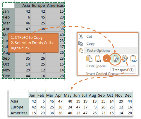
1. Copy > Paste Special > Transpose
The downside of Paste Special > Transpose
It’s really only good for one-time use since it’s not linked to the original data. That means if the original data is updated you’ll have to do the whole Copy > Paste Special > Transpose all over again, and manual repetition is Excel blasphemy.
2. Use a formula like the built in TRANSPOSE Function
TRANSPOSE is a multi-cell array function and as such you enter it with CTRL+SHIFT+ENTER like any other array formula.
The TRANSPOSE function only has one argument:
=TRANSPOSE(array)
Where ‘array’ is the range of cells you want to transpose.
First select the cells you want to place your transposed data in.
Tip: The trick here is knowing how big the range needs to be. I like to cheat a little and use the Copy > Paste Special > Transpose technique in step 1, and then with the pasted cells selected simply overwrite them with my TRANSPOSE formula.
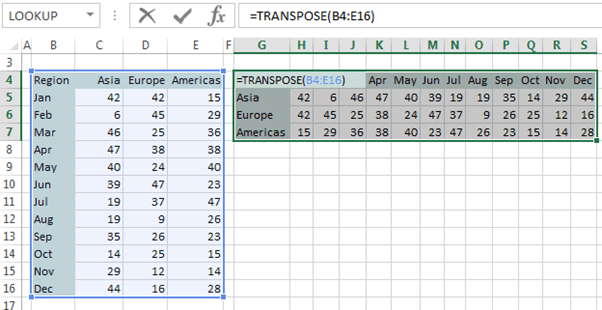
Don’t forget to press CTRL+SHIFT+ENTER to complete the formula.
The downside of the TRANSPOSE function:
If the size of the source data expands or contracts you have to manually update the formula. Yawn.
3. Use Power Query to Transpose Data
Power Query is available in Excel 2010 onwards so this technique isn’t for everyone (sorry 2007 users).
- Select your data > go to the Power Query tab (Excel 2016 see Get & Transform on the Data tab)
- Click the From Table icon
- Check Excel has correctly detected the range of your data (change if required) and uncheck the “My table has headers” box
- Click OK.
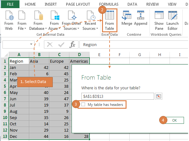
Note: If your data is already in an Excel Table you won’t see the above From Table dialog box.
Once you click OK the Power Query editor window will open and you’ll be able to see a preview of your data:
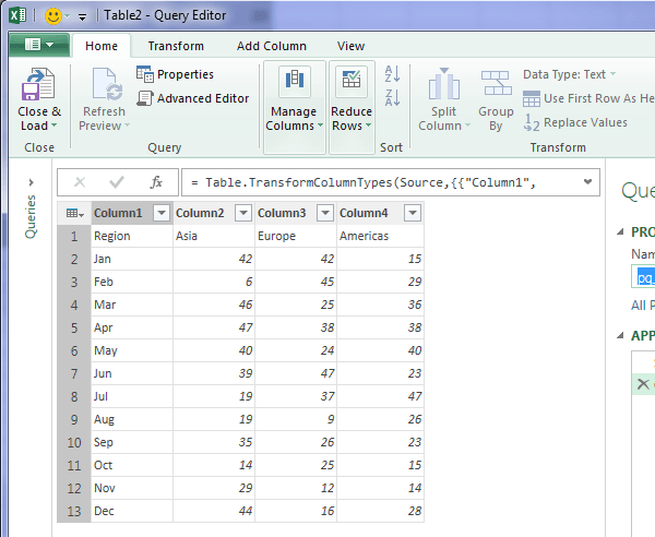
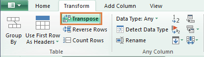
On the Transform tab in the Table group choose ‘Transpose’:
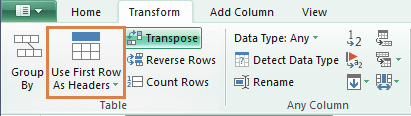
Then choose ‘Use First Row as Headers’:
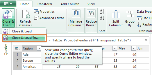
Now you’re ready to load your data back into Excel. On the Home tab > click ‘Close & Load To’:
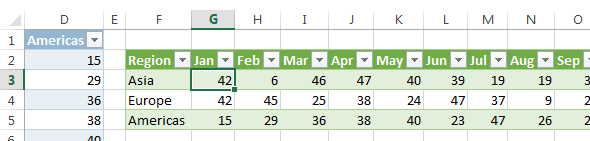
Choose where you want to put your data. I’ve put mine in the Excel worksheet beside my original data so you can see them together:
The downside of using Power Query
What? There’s no downside 😉
Ok, some might say it’s more complicated but it took me 25.62 seconds to complete the steps above (I had my son time me with the stop watch Santa bought him for Christmas so it must be accurate). And the best thing about using Power Query for transposing data is:
- If your table expands or contracts a simple refresh of the query will update the transposed data to incorporate any changes.
- I can get data from almost anywhere and transpose it, as well as loads of other data cleansing tasks I might want to do. For example, merge or split columns, unpivot, filter out duplicates and more. MUCH more.
Click here for more information on what Power Query can do, what versions of Excel it’s compatible with and information about our Power Query training.

You should also mention the VBA option!
Hi Sandeep,
Everything that’s built into Excel has a VBA option, but I don’t think we should use VBA unless it’s the last resort, only option.
Mynda
Hi Mynda,
2. Use a formula like the built-in TRANSPOSE Function
How do I add transpose in one cell at the same time highlighting the whole table?
Thank you
Hi Sally,
You can’t transpose a range of cells into a single cell. Perhaps you can post your question with a sample Excel file on our forum so we can see what you mean in context and help you from there.
Mynda
Aloha again.
Using Power Query this time, copied the table lower in the worksheet and added a new row to my data table (tblRegMon) and added region numbers. When I double clicked on the query, the Power Query window showed the expanded table. I was expecting the transposed data in the original worksheet to be updated (TRANSPOSE Function), but it wasn’t. And in the Power Query window, although the table was expanded with the added month, the “Close & Load” showed “Close and Load To” option grayed out, and the “Close and Load” option did not result in the transposed data set’s being expanded and loaded to the original worksheet.
in short, “If your table expands or contracts a simple refresh of the query will update the transposed data to incorporate any changes.” — how does the refresh update the transposed data in the original (i.e., not Power Query window) worksheet?
Mahalo (thanks)
Hi Jerald,
The sheet called ‘TRANSPOSE Function’ is not related/connected to the sheet called ‘Power Query Transpose’. The first one is for the formula example, and the second is for the Power Query example. If you copied the table (not sure which table you mean), then it may not be connected to the query at all.
Also note; Power Query doesn’t overwrite the original data/table. It creates its own table. Otherwise it would be in a never ending loop.
Close and Load ‘To’ is only available the first time you close and load the query. After that the ‘to’ option is only accessible by right-clicking the query in the ‘Workbook Queries’ pane > Load To.
Hope that makes sense, but if not please send me your file so I can see which table you copied and how it’s connected to Power Query.
Kind regards,
Mynda
Aloha. With the transpose array formula, you cannot turn the original data into a table (tblRegion) and then in the array formula use: transpose(tblRegion) ? When I do this, all I get transposed is “Jan” . . . I was hoping using a table as the data source would be more dynamic, but it seems not to be so.
Hi Jerald,
Good idea, but the Table structured references either refer to the headers, column(s) or row(s). There isn’t a structured reference for the entire range of the table (including the headers), which is why it won’t work with the TRANSPOSE function.
Mynda
Transpose Formula article great time saver, as Excel 2003 doesn’t include Transpose paste option.
Useful for rearranging DATA from Vertical to Horizontal for the purposes of Axis for creating CHARTS.
Excel doesn’t recognise Vertical Data for Plotting CHARTs, unless that’s just Excel 2003?
All your articles are clear & concise in purpose & formula.
Thanks, Stephan. Shame you still have Excel 2003.
Just wonderful as always.
Hoping to do the PowerQuery course.
Kind regards
Marg Pont
Thanks, Marg.
I’m sure you will love Power Query.
Mynda
I do a lot of transposing of data that may or may not be of the same number of cells, so I wrote a short VBA that transposes whatever data I copy and pastes only the values:
Sub TransVal()
‘ TransVal Macro
‘ Paste Transposed Values
Selection.PasteSpecial Paste:=xlPasteValues, Operation:=xlNone, SkipBlanks _
:=False, Transpose:=True
End Sub
I put up an icon on the Quick Access Toolbar, or if I am using it often in a file, place a button above the frozen pane.
Enjoy!
Thanks for sharing, Kevin 🙂
It’s not a comment but a question – is there a way to subtract a corresponding row or column from range of cells using Transpose formula?
E.g., Cells A1:E1 have values ins them. In cells A2:E2 I need ={Transpose(F1:F5)} minus a corresponding values in row 1. When I input =Transpose(F1:F5) – A1, the formula subtracts A1 from each cell, while I need it to be A1 from A2, B1 from B2, etc.
Appreciate your help
Hi Inna,
Yes, but your formula would be:
Entered with CTRL+SHIFT+ENTER as it’s an array formula.
Kind regards,
Mynda
For us poor relations still using 2007, there is another way, somewhere between 2 and 3:
Convert original data to a table and create a pivot table based upon it
It may not look as pretty without additional formatting and need refreshing to incorporate new data (but set refresh on open and you’re almost there)
New rows of data will be added on refresh but new columns will need dragging in
This was done in less than 10 seconds (I timed myself!)
But, of course, the reformatting would take several hours until you get it just right 😉
Hi Jim,
Of course, you can use Excel Tables as your PivotTable source and as new data is added to the Table a simple refresh will pick up the new data and incorporate it into the PivotTable.
Just note that the data has to be in a tabular format for the PivotTable to work with it.
Kind regards,
Mynda