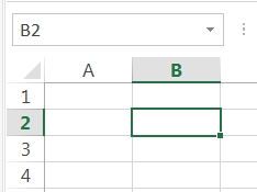
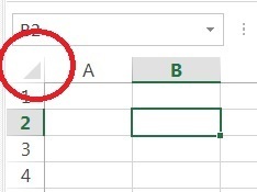
When you select a cell, or cells, in Excel, the row and column headers change color to indicate what you have selected. As you can see here we have selected B2. Or is it 2B? Hmm, 2B or not 2B?
If you have a busy sheet though, you may want a more obvious indication of your selection. One approach is to use conditional formatting to do this. However the problem with this is that it changes the formatting of the selected cells. Not good when you need that formatting.
So how do you Highlight Selected Cells in Excel and Preserve Cell Formatting? By using shapes.
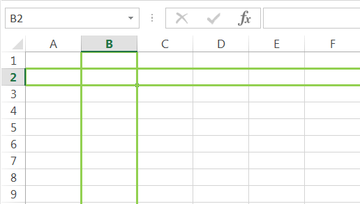
My approach is to draw shapes and overlay them on the column(s) and row(s) of the selected cell(s). Where these two shapes intersect is your selection.
You can use rectangles
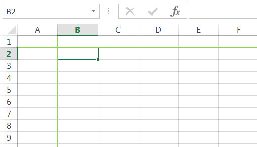
but these cover the fill handle and prevent it from being grabbed. You can alter the height of the box so that it is clear of the fill handle, or you could just use lines
To do this requires VBA, and we use a workbook event Workbook_SheetSelectionChange event. Essentially all we are doing is moving the shapes around as we click on different cells.
You don’t need to know any VBA to use this. I’ve written all the code. You just need to copy and paste and you can be using this on your workbooks.
You can download a sample workbook with all the code here :
Excel Workbook Using Rectangles.
Note: these are .xlsm files please ensure your browser doesn't change the file extension on download.
You can also get the code as plain text :
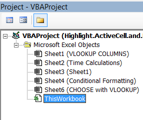
As we need this code to work in all sheets we enter the subroutine (macro) into the ThisWorkbook module. Every time we select a different cell, the VBA code is executed.
So How Does This Work?
The highlighting is achieved by drawing two rectangles, one over the cells in the selected row(s), and the other shape is drawn over the cell(s) in the selected columns(s). The intersection of the two shapes is your selection.
The first time we go to a sheet there won’t be any shapes so the VBA checks for the existence of the shapes, and draws them if they don’t exist. If you subsequently delete the shapes, or just one of them, they will be redrawn the next time you select a cell.
Special Selections
If you click on either a column or row header, Excel highlights that column or row in grey itself. So if this happens, the shapes are hidden by setting their .Visible property to FALSE. Next time you select a cell back on the sheet, the shapes are unhidden.
If you select the entire sheet either by CTRL+A or clicking the button at the top left of the sheet (between column header A and row header 1), the shapes are also hidden as Excel greys out the entire sheet. Just click back into a cell to see the shapes again.
If you select non-contiguous ranges, only the first range is highlighted. This may be something I can develop if there are enough requests for it.
Different Shape Formats on Different Sheets
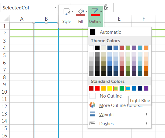
If your default shape format doesn’t happen to be particularly visible on a sheet, you can change the formatting of the shapes on that sheet to suit. You can actually have different shape formats on every sheet in your workbook if you like.
Select the shape and then right click. You can change the style, fill and outline from the right-click menu. You can go nuts and add shadows, reflections and glows but really that will be just visible noise. All you really need is to change the line color, weight and whether you want a dashed, dotted or solid line.
Once you change the shape format, the shape retains the new formatting until you either change it again, or delete the shape. Once you delete the shape, it will be redrawn (using your default formatting) when you next select a cell.
Fills
Don’t add a shape fill.
If you do the fill sits over any selected cells and you will probably end up clicking on the shape(s) all the time. With no fill, the shape becomes ‘hollow’ and allows you to click through it to the cells below.
Line Colors
I’m using an RGB (Red, Green, Blue) value to set my line color. When I set .Line.ForeColor.RGB = RGB(146, 208, 80) I get a nice green and you know we like green on this site.
You can set your own RGB values and can use this site to figure out RGB values for your own colors.
Alternatively you can use in-built Excel color constants vbBlack, vbWhite, vbRed, vbGreen, vbBlue, vbYellow, vbMagenta, vbCyan so .Line.ForeColor.RGB = vbMagenta will give your shape magenta lines.
Changing the Default Shape Style
There are two section of code like this, one for the RowShape and one for the ColShape. These control how the shapes look when they are first drawn. If you don't like it then adjust the settings here.
The .Line.Weight value sets the thickness of the lines. I've got it at 2.
.Line.ForeColor.RGB specifies the RGB values for the color of the boxes.
If you don't like the default line style of a solid, continuous line, you can specify a value for .DashStyle. I've got it commented out (the apostrophe at the start of the line) as the default is a solid line and I am happy with that.
For the method using just lines, you can similarly adjust the line weight and color.
Shape Size
Shapes are drawn to the size of the visible range. What this means is that the shapes will extend from the left to the right of the visible cells in the sheet, and from the top to the bottom of the visible cells. Basically the shapes will be drawn to the edges of what you can see of your worksheet.
If you then zoom out, you’ll see the extent of the shapes. Click in another cell when zoomed out and the shapes redraw to fit your screen again.
The same thing will be noticed if you save the workbook on a computer with a small screen, and then open it on a computer with a large screen. But as soon as you click into a cell, the shapes are redrawn to fit the screen.
The Code
Enter your email address below to download the sample workbook.
You can download a workbook with the code in it from here. I've tested this in Excel 2010 and 2013.
Excel Workbook Using Rectangles
You can also get the code as plain text :
Private Sub Workbook_SheetSelectionChange(ByVal Sh As Object, ByVal Target As Range)
' Written by Philip Treacy
' myonlinetraininghub.com/highlight-selected-cells-in-excel-and-preserve-cell-formatting
'
Dim RowShape As Shape, ColShape As Shape
' ************************************************
' Check if entire rows or columns are selected
' If they are then hide the shapes
' ************************************************
If Target.Address = Selection.EntireRow.Address Then
'If error occurs because shape does not exist, ignore the error
On Error Resume Next
Sh.Shapes("SelectedRow").Visible = msoFalse
Sh.Shapes("SelectedCol").Visible = msoFalse
'Return error handling to Excel
On Error GoTo 0
Exit Sub
End If
If Target.Address = Selection.EntireColumn.Address Then
'If error occurs because shape does not exist, ignore the error
On Error Resume Next
Sh.Shapes("SelectedCol").Visible = msoFalse
Sh.Shapes("SelectedRow").Visible = msoFalse
'Return error handling to Excel
On Error GoTo 0
Exit Sub
End If
' ************************************************
' ************************************************
' Create shapes on active sheet if they don't exist
' ************************************************
' Set RowShape and ColShape to be the
' SelectedRow and SelectedCol shapes respectively
On Error Resume Next
Set RowShape = Sh.Shapes("SelectedRow")
Set ColShape = Sh.Shapes("SelectedCol")
On Error GoTo 0
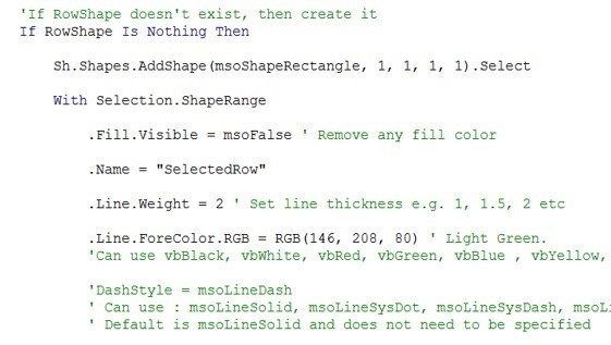
'If RowShape doesn't exist, then create it
If RowShape Is Nothing Then
Sh.Shapes.AddShape(msoShapeRectangle, 1, 1, 1, 1).Select
With Selection.ShapeRange
.Fill.Visible = msoFalse
.Name = "SelectedRow"
.Line.Weight = 2
.Line.ForeColor.RGB = RGB(146, 208, 80) ' Light Green.
'
'Can use vbBlack, vbWhite, vbRed, vbGreen,
'vbBlue , vbYellow, vbMagenta, vbCyan
End With
End If
'If ColShape doesn't exist, then create it
If ColShape Is Nothing Then
Sh.Shapes.AddShape(msoShapeRectangle, 1, 1, 1, 1).Select
With Selection.ShapeRange
.Fill.Visible = msoFalse
.Name = "SelectedCol"
.Line.Weight = 2
.Line.ForeColor.RGB = RGB(146, 208, 80) ' Light Green
End With
End If
' ************************************************
' ************************************************
' Move the SelectedRow and SelectedCol shapes
' ************************************************
With Sh.Shapes("SelectedRow")
'Make sure it is visible, may be hidden by previous selection
.Visible = msoTrue
.Top = Target.Top
.Left = ActiveWindow.VisibleRange.Left
.Width = ActiveWindow.VisibleRange.Width
.Height = Target.Height
End With
With Sh.Shapes("SelectedCol")
'Make sure it is visible, may be hidden by previous selection
.Visible = msoTrue
.Top = ActiveWindow.VisibleRange.Top
.Left = Target.Left
.Width = Target.Width
.Height = ActiveWindow.VisibleRange.Height
End With
' ************************************************
' Must do this to stop shape being selected if navigating with cursor keys
Target.Select
End Sub
Hello,
Is it possible to add this code to a module and set a shortcut key for it too?
Hi Wansley,
Press Alt+F8 keys, this will open the macro dialog. Select a macro from list, Click the Options button, this will allow you to set a shortcut key to run that macro.
HI,
I like this code, but can it be changed to highlight only one cell with thick border in RED? (not the whole row and column)
Sure can George, here’s the code
Highlight With Red Box
Regards
Phil
Thank you 🙂
No worries
hi Could you please give me a code wherein it works only one one specific worksheet rather than whole workbook and it does not convert/change or fill the cells with colour. I want it to highlight without altering the already existing conditional formatting. when the cell is selected it should highlight without blocking the view of the data.
thanks,
Hi,
To use it only on a specific sheet, it’s easy. Just add this line after the line Private Sub Workbook_SheetSelectionChange(ByVal Sh As Object….:
If Not Sh.Name like “Sheet1” then exit sub
See the comments below for variations of this code, that can allow you to draw the shapes right outside the borders, so the lines are not within the cells limits, it will not block the view.
Catalin
Great Job. Nice idea to work with shapes!
But..
It doesn’t work as you freeze pane. the shape doesn’t appear on the frozen columns or rows.
Hi Didier,
If you scroll a bit down, you will see the solutions that will work on frozen panes also, it involves removing VisibleRange from codes.
Regards,
Catalin
Hi Phil, amazing code. Just as a comment and if you want to burn your mind in programming a little more, just two issues found in this code:
1. When freezing panes it mess the selection. Just creates the line on the visible area. It would be great if it was possible to make the row line in the whole line of the spreadsheet like when we do SHIFT+SPACE. I saw the other post to remove the .visible, and I did, and solved the pane thing, but the with doesn’t cover all cells as we do when hitting SHIFT+SPACE. How could be the command for width to get the whole line ;
2. Not sure if it is possible, is to make the “Green” line to be on the back (behind) the selected cell, because the way it is now, it isn’t possible to select/pick the fill handle (+) on the corner of the cell to do commands like repeat values by dragging or the increment values. Not big deal because there is a workaround by selecting the “green” line, moving it to the side and going back to the cell to click on the handle (+). But if it was possible to make the lines behind, the workaround wouldn’t be necessary.
Thanks and have a nice day
Hi Lucato,
I assume you are using the version with green rectangles. I think you should try the version with lines instead of rectangles, to be able to use the fill handle.
Or, you can make your own flavor, resizing the rectangles to be smaller than the cell size:
With Sh.Shapes(“SelectedRow”)
.Visible = msoTrue ‘Make sure it is visible, it may have been hidden by previous selection
.Top = Target.Top + 5
.Left = ActiveWindow.VisibleRange.Left + 10
.Width = ActiveWindow.VisibleRange.Width – 20
.Height = Target.Height – 10
End With
With Sh.Shapes(“SelectedCol”)
.Visible = msoTrue ‘Make sure it is visible, it may have been hidden by previous selection
.Top = ActiveWindow.VisibleRange.Top + 5
.Left = Target.Left + 10
.Width = Target.Width – 20
.Height = ActiveWindow.VisibleRange.Height – 10
End With
Hi Phill, thanks for your reply I’ll try it out. Just adding, I found one issue. By using “the code” excel doesn’t allow to UNDO, so I lose all undo function. Any idea how to fix it in the code? Thanks.
Regarding the code with -10 +5 and so on, they solve the fill handle, but not the other 2 issues: (1) Freezing panes, e UNDO.
Thanks.
Hi,
You have to combine the solution with removing VisibleRange from code, as described here.
Or, try a different approach, without shapes, proposed by Rick Rothstein
For UNDO, there is a method that will not clear the clipboard, as UNDO relies on that information to perform the undo:
Use this:
Option Explicit
Private Declare Function OpenClipboard Lib “User32” _
(ByVal hwnd As Long) As Long
Private Declare Function CloseClipboard Lib “User32” () As Long
At the beginning of the code, use this line, it will kep the clipboard open while the code is running, this way it will not be cleared:
OpenClipboard 0
Then, before End Sub, simply close the clipboard with:
CloseClipboard
This should allow you to use whatever you have in clipboard, for undo, copy paste, and so on.
Catalin
Hi Lucato,
When you run a macro (any macro) Excel does not record what the macro did. So Undo is not available to rewind whatever it is the macro did.
Unfortunately that’s the way Excel works.
Phil
Hi Phil & Catalin, thanks for the reply I appreciated that.
@Phil what a pity, it is terrible, because after hitting enter in the cell, there is no way to undo the value or if you have deleted a cell, there is no way to undo the mistake!
@Catalin
Regarding the freezing panes I tried the method you linked, and didn’t work and the 2nd link I have colored things, so didn’t fit for my needs, but the solution I got by myself was to change a value at .Widht, so I have replaced the value to “.Width = 40000” and worked and the line/rectangle goes through the freezing panes. ;0)
Regarding the UNDO, it didn’t work, actually, I’m very newbie in VBA, so I’m not sure if I understood your code and placed the lines/commands in the right place, so here is how I did:
Option Explicit
Private Declare Function OpenClipboard Lib “User32” (ByVal hWnd As Long) As Long
Private Declare Function CloseClipboard Lib “User32” () As Long
_________________________________________________________
Private Sub Workbook_SheetSelectionChange(ByVal Sh As Object, ByVal Target As Range)
OpenClipboard 0
Dim RowShape As Shape
‘ ************************************************
‘ Check if entire rows are selected
‘ If they are then hide the shapes
‘ ************************************************
If Target.Address = Selection.EntireRow.Address Then
‘If error occurs because shape does not exist, ignore the error
On Error Resume Next
Sh.Shapes(“SelectedRow”).Visible = msoFalse
‘Return error handling to Excel
On Error GoTo 0
Exit Sub
End If
If Target.Address = Selection.EntireColumn.Address Then
‘If error occurs because shape does not exist, ignore the error
On Error Resume Next
Sh.Shapes(“SelectedCol”).Visible = msoFalse
Sh.Shapes(“SelectedRow”).Visible = msoFalse
‘Return error handling to Excel
On Error GoTo 0
Exit Sub
End If
‘ Set RowShape to be the SelectedRow
On Error Resume Next
Set RowShape = Sh.Shapes(“SelectedRow”)
On Error GoTo 0
‘If RowShape doesn’t exist, then create it
If RowShape Is Nothing Then
Sh.Shapes.AddShape(msoShapeRectangle, 1, 1, 1, 1).Select
‘Sh.Shapes.AddLine(1, 1, 1, 1).Select
With Selection.ShapeRange
.Fill.Visible = msoFalse ‘ Remove any fill color
.Name = “SelectedRow”
.Line.Weight = 2 ‘ Set line thickness e.g. 1, 1.5, 2 etc
.Line.ForeColor.RGB = RGB(158, 0, 0) ‘ Light Green.
‘Can use vbBlack, vbWhite, vbRed, vbGreen, vbBlue , vbYellow, vbMagenta, vbCyan
‘ DashStyle = msoLineLongDash
‘ Can use : msoLineSolid, msoLineSysDot, msoLineSysDash, msoLineDash, msoLineDashDot, msoLineLongDash, msoLineLongDashDot, msoLineLongDashDotDot
‘ Default is msoLineSolid and does not need to be specified
End With
End If
‘ ************************************************
‘ Move the SelectedRow shape
‘ ************************************************
With Sh.Shapes(“SelectedRow”)
.Visible = msoTrue ‘Make sure it is visible, it may have been hidden by previous selection
.Top = Target.Top – 5
.Left = ActiveWindow.Left
.Width = 40000 ‘ActiveWindow.Width – 20
.Height = Target.Height + 10
End With
Target.Select
CloseClipboard
End Sub
Thanks you all and have a great weekend.
Hi Lucato,
Opening the clipboard when running codes will simple lock the clipboard, this will not allow vb to clear the clipboard, you will still have in clipboard what you previously copied.
Undo is different, there is no way to preserve the undo stack when running any vba codes.
Hi Phil,
Thanks for your valuable study. There is a small problem that I have faced when using the freeze panes. the forozen cells cannot be highlighted. Could you show me the solution?
Regards,
Onur
Hi Onur,
Try removing the .VisibleRange property from the following lines of code:
.Left = ActiveWindow.VisibleRange.Left
.Width = ActiveWindow.VisibleRange.Width
.Top = ActiveWindow.VisibleRange.Top
.Height = ActiveWindow.VisibleRange.Height
It should look like: .Left = ActiveWindow.Left
Catalin
Hi There,
I have frozen panes for row and column. I tried modifying it by removing all the “VisibleRange” but it doesn’t work making the shape for row gone.
I use the code below and the shape for the column worked but the shape for the row stopped where I proze the panes.
With Sh.Shapes(“SelectedRow”)
.Visible = msoTrue ‘Make sure it is visible, it may have been hidden by previous selection
.Top = Target.Top
.Left = ActiveWindow.VisibleRange.Left
.Width = ActiveWindow.VisibleRange.Width
.Height = Target.Height
End With
With Sh.Shapes(“SelectedCol”)
.Visible = msoTrue ‘Make sure it is visible, it may have been hidden by previous selection
.Top = ActiveWindow.Top
.Left = Target.Left
.Width = Target.Width
.Height = ActiveWindow.Height
End With
What can be the possible solution here to make the shape for the row go inside the frozen panes? Please help. Thanks.
Remove .VisibleRange from row too, not only for column then, I can see in your code that you still have .VisibleRange in With Sh.Shapes(“SelectedRow”) code.
Phil, I love the code and the possibilities it provides; however I am getting some mixed reactions when I move around within different files. The two file types I am using are xlsx and xlsm. I have files of both type that work flawlessly. I also have files of both type that either don’t work at all or the crosshairs are not on the selected cell. The ones that don’t work are causing errors with the sh variable. I added the code you provided but it still won’t work. In some files the crosshairs don’t line up with selected cell, but it will be correct when you go to a different tab in that same file, but a third tab might not work as well.
L.E.: Also, is there a way to assign this to a button so I could turn it on and off as desired?
Thanks,
Will
Hi Will,
Can you create a sample workbook that does not work and upload it on our forum? It’s hard to see a reason without testing your file.
To turn the code on and off, you can add somewhere in your workbook a dropdown with 2 values: Enabled and Disabled. Define a name for this cell, EnableCode for example.
Then you can add a simple line of code at the beginning of the code to check this named range value:
If Worksheets(“Sheet1”).Range(“EnableCode”) =”Disabled” Then Exit Sub
I removed it because it was printing and not when I put it back it doesn’t run on any files. Not sure what’s up with that.
By the button idea I meant a button on my toolbar so I could control it on/off for whatever file I was in.
Will
Hi Will,
A setting that should work from anywhere should use a registry key to store a parameter.
Here is how you can create a registry key that can be called from any code:
Public Function GetCodeSetting(Name As String, Optional DefaultValue) As String

    GetCodeSetting = VBA.Interaction.GetSetting("Enable Code", "Preferences", Name, DefaultValue)

End Function
Public Function SetCodeSetting(Name As String, NewValue As String)

    VBA.Interaction.SaveSetting "Enable Code", "Preferences", Name, NewValue

End Function
Sub EnableCode()

SetCodeSetting "CodeSetting", True

End Sub

Sub DisableCode()

SetCodeSetting "CodeSetting", False

End Sub
Sub Test()
EnableCode
MsgBox "Enabled: " & GetCodeSetting("CodeSetting")
DisableCode
MsgBox "Disabled: " & GetCodeSetting("CodeSetting")
End Sub
The only thing you should make sure you do is to use the Wotkbook_Open event to create the registry key, otherwise when you try to get the setting, it will fail:
Private Sub Workbook_Open()

SetCodeSetting "CodeSetting", True

End Sub
This means that when you open the workbook, the setting is True by default.
Next thing you should do is to add te buttons on Quick Access toolbar, to turn code on and off. See this article for a method to do that: customize-the-qat-in-excel
The buttons should refer to the EnableCode and DisableCode from above.
You can also run the Test procedure, you will see how it works.
Now, your code to highlight selected cells can be turned off with a simple code that reads the registry setting, placed at the beginning of your code:
If GetCodeSetting("CodeSetting")=False Then Exit Sub
I’m very green to VBA’s but then anyone get this to work and if so can you explain this to me. I’m having a hard time understand where i should put the VBA code.
Hi Wansley,
The code should be in ThisWorkbook module. Press Alt+F11 to open the visual basic editor, you will see there on the left side the project explorer panel, double click on those modules listed under the project and on the right side you will see the codes from that module.
Use the files that are provided for download, to see the codes.
The fixes from comments will replace parts of the code, as described in that comment.
Hello Catalin,
Thank you for assistance. I added the code plus the additional comment addons(please see below) and when i run the test macro the enable is true but disable false. Is there something wrong with the way I added the code?
Private Sub Workbook_SheetSelectionChange(ByVal Sh As Object, ByVal Target As Range) ' Written by Philip Treacy, https://www.myonlinetraininghub.com/highlight-selected-cells-in-excel-and-preserve-cell-formatting ' Dim RowShape As Shape, ColShape As Shape ' ************************************************ ' Check if entire rows or columns are selected ' If they are then hide the shapes ' ************************************************ If Target.Address = Selection.EntireRow.Address Then 'If error occurs because shape does not exist, ignore the error On Error Resume Next Sh.Shapes("SelectedRow").Visible = msoFalse Sh.Shapes("SelectedCol").Visible = msoFalse 'Return error handling to Excel On Error GoTo 0 Exit Sub End If 'If Target.Address = ActiveCell.EntireColumn.Address Then If Target.Address = Selection.EntireColumn.Address Then 'If error occurs because shape does not exist, ignore the error On Error Resume Next Sh.Shapes("SelectedCol").Visible = msoFalse Sh.Shapes("SelectedRow").Visible = msoFalse 'Return error handling to Excel On Error GoTo 0 Exit Sub End If ' ************************************************ ' ************************************************ ' Create shapes on active sheet if they don't exist ' ************************************************ ' Set RowShape and ColShape to be the SelectedRow and SelectedCol shapes respectively On Error Resume Next Set RowShape = Sh.Shapes("SelectedRow") Set ColShape = Sh.Shapes("SelectedCol") On Error GoTo 0 'If RowShape doesn't exist, then create it If RowShape Is Nothing Then Sh.Shapes.AddShape(msoShapeRectangle, 1, 1, 1, 1).Select With Selection.ShapeRange .Fill.Visible = msoFalse ' Remove any fill color .Name = "SelectedRow" .Line.Weight = 2 ' Set line thickness e.g. 1, 1.5, 2 etc .Line.ForeColor.RGB = RGB(146, 208, 80) ' Light Green. 'Can use vbBlack, vbWhite, vbRed, vbGreen, vbBlue , vbYellow, vbMagenta, vbCyan 'DashStyle = msoLineDash ' Can use : msoLineSolid, msoLineSysDot, msoLineSysDash, msoLineDash, msoLineDashDot, msoLineLongDash, msoLineLongDashDot, msoLineLongDashDotDot ' Default is msoLineSolid and does not need to be specified End With End If 'If ColShape doesn't exist, then create it If ColShape Is Nothing Then Sh.Shapes.AddShape(msoShapeRectangle, 1, 1, 1, 1).Select With Selection.ShapeRange .Fill.Visible = msoFalse .Name = "SelectedCol" .Line.Weight = 2 .Line.ForeColor.RGB = RGB(146, 208, 80) ' Light Green End With End If ' ************************************************ ' ************************************************ ' Move the SelectedRow and SelectedCol shapes ' ************************************************ With Sh.Shapes("SelectedRow") .Visible = msoTrue 'Make sure it is visible, it may have been hidden by previous selection .Top = Target.Top .Left = ActiveWindow.VisibleRange.Left .Width = ActiveWindow.VisibleRange.Width .Height = Target.Height End With With Sh.Shapes("SelectedCol") .Visible = msoTrue 'Make sure it is visible, it may have been hidden by previous selection .Top = ActiveWindow.VisibleRange.Top .Left = Target.Left .Width = Target.Width .Height = ActiveWindow.VisibleRange.Height End With ' ************************************************ Target.Select ' Must do this to stop shape being selected if navigating with cursor keys End Sub Public Function GetCodeSetting(Name As String, Optional DefaultValue) As String GetCodeSetting = VBA.Interaction.GetSetting("Enable Code", "Preferences", Name, DefaultValue) End Function Public Function SetCodeSetting(Name As String, NewValue As String) VBA.Interaction.SaveSetting "Enable Code", "Preferences", Name, NewValue End Function Sub EnableCode() SetCodeSetting "CodeSetting", True End Sub Sub DisableCode() SetCodeSetting "CodeSetting", False End Sub Sub Test() EnableCode MsgBox "Enabled: " & GetCodeSetting("CodeSetting") DisableCode MsgBox "Disabled: " & GetCodeSetting("CodeSetting") End Sub Private Sub Workbook_Open() If GetCodeSetting("CodeSetting") = False Then Exit Sub SetCodeSetting "CodeSetting", True End SubHi Wansley,
Can you please upload a sample file on our forum and a more clear description of what happens, not sure what you mean by: “when i run the test macro the enable is true but disable false”
Hello.
This is brill.
Q – How can I apply this to one sheet in a workbook only? As your code seemed to only work globally when added to the ThisWorkbook VBA object.
I tried copying it into a worksheet selection event but it bugs out. Wanted me to define sh (which I did as an object) then gave an error Object variable or With block variable not set
Fairly new to VBA so any advice greatly appreciated.
Thanks
Hi,
After the first line:
Private Sub Workbook_SheetSelectionChange(ByVal Sh As Object, ByVal Target As Range)
Wrap the rest of the code into an If statement, that will work only when the change is triggered from that sheet:
If Sh.Name=”Sheet1″ Then
‘ rest of code
end if
Catalin
This is so cool! Thank you very much!
You’re welcome
Hello, Nice Code, i would like to change the color, i have read the code, and when i change the RGB color, the lines color doesnt change at all, i have tried multiple values for RGB and nothing changes.
What to do?
Hi,
Sorry about that. The line colour is only set when the line is initially drawn. So the quickest way to see your colour change would be to delete the line from the sheet.
When you then select something, the line will be redrawn with the new colour.
For a different fix, you can add 2 lines of code. Just before the section titled ‘Move the SelectedRow and SelectedCol shapes’ add this:
Regards
Phil
If you do not have a lot of colored cells on your worksheet, perhaps this alternate code will prove useful. What it does is color all non-colored cells horizontally and vertically from the selected cell(s) yellow (actually, 1 less than the value for vbYellow so that the code will leave yellow cells untouched)…
Private Sub Worksheet_SelectionChange(ByVal Target As Range)
Application.FindFormat.Clear
Application.ReplaceFormat.Clear
Application.FindFormat.Interior.Color = 65534 ‘one less than vbYellow’s value
Application.ReplaceFormat.Interior.Color = xlNone
Cells.Replace “”, “”, SearchFormat:=True, ReplaceFormat:=True
Application.FindFormat.Clear
Application.ReplaceFormat.Clear
Application.FindFormat.Interior.Color = xlNone
Application.ReplaceFormat.Interior.Color = 65534 ‘one less than vbYellow’s value
Target.EntireRow.Replace “”, “”, SearchFormat:=True, ReplaceFormat:=True
Target.EntireColumn.Replace “”, “”, SearchFormat:=True, ReplaceFormat:=True
Application.FindFormat.Clear
Application.ReplaceFormat.Clear
End Sub
Thanks Rick.
Regards
Phil
Phil,
I was looking for a solution like this, specifically to highlight rows. This was easy to change. But like other posters suggested: I want it to be available in all my workbooks, but only when I want to use it.
I solved it like this, and I hope that posting it here can help others:
I’ve replaced the routine
Private Sub Workbook_Open()
Set App = Application
End Sub
With the following routine
Public Sub Highlight_Activate()
Dim Rowshape As Shape
Dim sh As Worksheet, Target As Range
Set sh = ActiveWorkbook.ActiveSheet
Set Target = ActiveCell
On Error Resume Next
Set Rowshape = sh.Shapes(“SelectedRow”)
On Error GoTo 0
If Rowshape Is Nothing Then
Set App = Application
sh.Shapes.AddShape(msoShapeRoundedRectangle, 1, 1, 1, 1).Select
With Selection.ShapeRange
.Name = “SelectedRow”
.Fill.Visible = msoFalse
.Line.Weight = 2
.Line.ForeColor.RGB = RGB(146, 208, 80)
End With
With sh.Shapes(“SelectedRow”)
.Visible = msoTrue ‘Make sure it is visible, it may have been hidden by previous selection
.Top = Target.Top
.Left = ActiveWindow.VisibleRange.Left
.Width = ActiveWindow.VisibleRange.Width
.Height = Target.Height
End With
Else
Set App = Nothing
Rowshape.Delete
End If
End Sub
Then I added the macro (which is now available for selection from personalxlsb!.ThisWorkbook because it is public) to my personal tab on the ribbon. Now if I click it and the shape SelectedRow does not yet exist, it is created on the ActiveCell row and wil move with every new selection.
When I click my macrobutton again the shape is deleted and the app is set to Nothing: I can select without a shape following me around!
As I said, I hope others can benefit.
Cheers,
Stefan van Gaal
Great, thanks Stefan.
Phil
Phil, I think this is amazing! Is it possible to combine Mark D and Andrew’s requests for the best of all possible worlds? I would love to have a version with lines in my Personal.xlsb. Thanks so much for the great tips!
Thanks Roxie.
Try this, it will work for ALL workbooks, and uses lines. I haven’t chnaged the width/height of the lines yet though. So they are still just drawn to the extent of the visible sheet, but that will be the next thing I work on.
You can download the code in text from here.
Paste it into the ThisWorkbook module of Personal.xlsb and restart Excel.
Regards
Phil
I often use Excel to examine output data from my sql scripts and this looked to be a major help when I’m scrolling around some of the large flat files but by overlaying shapes prevents you doing things like grabbing the autofill handle which I use to populate data validation/exception formulae.
The restriction limiting the shape to the visible screen is also an issue when scrolling around and you’re trying to read across a record with a hundred or more data fields.
You’ve given me food for thought, perhaps instead of 2 rectangles, 2 lines, one across the top of the selected cell and one to the left, both extending to the full spreadsheet.
Hi Mark,
Good points. Using a couple of lines instead of boxes is a simple modification and you can get the code here. This has one line along the left of the cell and one along the top as you suggested, so the selected cell is always below and to the right of the line intersection, leaving the fill handle accessible.
Altering the width and height of these shapes should be pretty straightforward too. I haven’t done this in the above modified file, but will look at this as soon as I can.
Regards
Phil
Absolutely love the crosshairs! I think this could be super useful for navigating rows of data; I often-times have to hit CTRL+SPACE or ALT+SPACE to help my eyes when scrolling across rows and columns. I tried adding this to my personal macro workbook, but it didn’t work. Is there a way to format the code so that it’s a executable macro, rather than something which must be embedded in every excel workbook you want it in?
Thanks Andrew. To make this work for every workbook you do put the code into Personal.xlsb but you have to modify it slightly.
The code needs to make use of application events, rather than the workbook events we are using right now. Essentially you are telling Excel to pass the workbook level events up to the application event handler in Personal.xlsb.
This results in events that the workbook itself would normally deal with (the workbook level), being dealt with by code you write to execute for all workbooks (the application level).
I’ve modified the code and you can download it in text format here. Copy and paste the code from this text file into the ThisWorkbook module in Personal.xlsb.
Then close and restart Excel and it should work for all workbooks.
Let me know if you have any issues.
Regards
Phil
Phil,
I’m running into issues implementing this code into a personal workbook that already has your brilliant lock/unlock macros. I have tried adding a module but it replaces what is already there. I tried insert module and that gave me a compile error. Is there a trick to using multiple modules in your personal.xlsb?
Thanks!
Hi Jeanette,
To make this code work in Personal.xlsb it has to be modified a bit. As we are using workbook level events, the code is usually placed into the ThisWorkbook module of the workbook. This code they won’t be triggered in Personal.xlsb unless we instruct Excel to do so and place it into Personal.xlsb.
Please note that implementing this code in Personal.xlsb will mean the code works for ALL workbooks, which you may not want. I’m working on some code to get around this.
I’ve got two versions of the code for Personal.xlsb, one using rectangles and the other using lines.
Here’s a link to the rectangles (this is a .xlsm)
and here’s the lines (this is a text file)
This code must go into the ThisWorkbook module of Personal.xlsb.
Let me know if you have any issues.
Phil
Hi Phil,
I’d love to have this macro work for each and every sheet. I tweaked its appearance to have less bolt format to be less “intrusive” 😉 however it’s great.
Just I don’t understand how to make this working on all files I may open.
FYI, I have copied the routine into the “This Workbook” of my Personal.xlsb however it appears to work on the personal w/b itself, only.
Would there plase be a chance to have some .xlam file I can add to the Add-ins?
Many thanks in advance,
Regards,
Giuseppe
Hi Giuseppe,
A few other commenters have asked the same thing. If you look in my other comment replies I’ve linked to code to make this run for all workbooks.
The code does go into ThisWorkbook in PERSONAL.XLSB, but need some modification to work. But I’ve done all of that already.
Let me know if you have trouble getting it to work.
Cheers
Phil
Hi Phil,
I recently installed MO2016 and since then I’ve run into the issue below.
When I open some files (could be either .xlsx or .xlsb) and I click on any cells it gives me this error:
Run-Time error ‘1004’:
Application-defined or object-defined error
and debugger brings me to:
Sh.Shapes.AddLine(1, 1, 1, 1).Select
Then I need to restart again Excel hoping not to open any “wrong” file. What could be the issue with such files?
Thanks in advance.
Kind Regards
Giuseppe
Hi Giuseppe,
If the code is erroring there, I’m guessing it’s because the Sh object is not set. But I’m not sure how that happens as Sh should contain the worksheet.
Try adding this line to the top of the Workbook_SheetSelectionChange
Phil
Can you recreate this problem with the same file(s) over and over again? If so can you send me some of these files so I can test them?