Last week I showed you how you can extract a list that excludes blank cells for use in a data validation list.
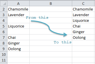
Using this array formula in cells C2:C10:
=IFERROR(INDEX($A$2:$A$10,SMALL(IF(ISTEXT($A$2:$A$10),ROW($A$1:$A$9),""), ROW(A1))),"")
Aside: Roberto from Excel blog E90E50 pointed out to me that we can actually leave out the "" from the SMALL(IF part of the formula as the SMALL function doesn’t consider the Boolean values. So we can shorten the formula to this:
=IFERROR(INDEX($A$2:$A$10,SMALL(IF(ISTEXT($A$2:$A$10),ROW($A$1:$A$9)), ROW(A1))),"")
Entered with CTRL+SHIFT+ENTER as it’s an array formula.
OK moving on, now that we have a list in column C without blanks we want to use it as the Source of our Data Validation List, and we want to allow for growth in the list, which means it needs to be dynamic.
It’d be nice if we could use one of the ways to create dynamic named ranges I showed you a couple of weeks ago, but we can’t 🙁
This is because those examples use the COUNTA function, and COUNTA counts blanks returned from formulas.
Which means it would include cells C8:C10 because although they appear blank they actually evaluate to blank using the IFERROR part of the formula.
When a Blank Cell Isn’t Really Blank
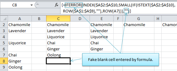
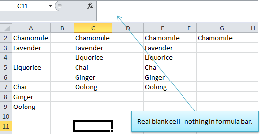
We therefore need to use a slightly different formula that excludes blank cells (both real and fake) from the count.
Note: ‘fake blank cell’ is not a technical term :).
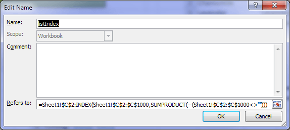
Exclude Blanks in a Dynamic Named Range
We can use the following formula to dynamically calculate the named range that excludes both fake blank cells (blanks generated from a formula), and real blank/empty cells:
=Sheet1!$C$2:INDEX(Sheet1!$C$2:$C$1000,SUMPRODUCT(--(Sheet1!$C$2:$C$1000<>"")))
In English this reads:
Return a range that starts in cell C2 through to the last cell in the range C2:C1000 that isn’t blank.
Which evaluates to:
Sheet1!$C$2:$C$7
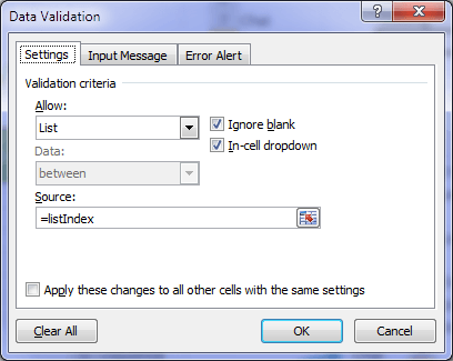
We can give the formula a name (listIndex) in the name manger:
And use the name as the source for our Data Validation list:
Let’s inspect this formula a little closer:
=Sheet1!$C$2:INDEX(Sheet1!$C$2:$C$1000,SUMPRODUCT(--(Sheet1!$C$2:$C$1000<>"")))
The starting point of the range is fixed:
Sheet1!$C$2:
The second part is resolved using the INDEX function.
Remember the syntax for INDEX is:
=INDEX(reference, row_num, [column_num], [area_num])
And we’re only using the first two arguments in this formula.
First the SUMPRODUCT part:
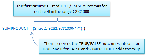
Our formula therefore evaluates SUMPRODUCT like this:
=Sheet1!$C$2:INDEX(Sheet1!$C$2:$C$1000,6)
Since there are 6 cells in the range C2:C1000 that are not blank.
And since C7 is the 6th in the range C2:C1000 INDEX evaluates like this:
=Sheet1!$C$2:$C$7
Download the workbook
Enter your email address below to download the sample workbook.
Bonus: See sheet ‘r’ in this workbook for an alternative solution provided by Roberto that hides errors using conditional formatting instead of IFERROR, and therefore uses a different formula for the named range used in the data validation list.
Thanks for sharing, Roberto 🙂


Hi! so what if I just want to generate a column with all the text in another column generated by formulas? I mean, those blanks are not real blanks as you described, but I would like to generate another column where it only shows the result where it’s not ” “. Is that possible?
Hi Kevin,
I’m not sure I follow you because I think that’s what the formula above does i.e. generate a list of values ignoring the blanks. If you have Microsoft 365 or Excel 2021, you can use the FILTER function, which won’t give you false blanks with “”.
Mynda
I am trying to use this in conjunction with a dropdown list that utilized the “=INDIRECT” function.
In the Name Manager, I see that the value of the named range is shown as {,,,}. When I set the dropdown list equal to the name, there is no issue (all the values show up without blanks). When I try to use the “=INDIRECT” function, an error occurs and I can’t select any items from the dropdown list.
Hi Nathan,
Can you upload a file with the formulas you are using, to see what you are saying?
You can use our forum to create a new topic for upload.
Excel Forum
Spot on, stuff like this makes life so much better 🙂
Great to hear, Craig!
AWESOME! … Exactly what I’ve searched for.
Thank you so much 😀
Glad it was helpful, Markus!
Thank you, this works very well.
I was wondering if you have an idea how to extend the formula a little bit to be able to do the following:
Let’s say column B has a number behind every tea type in column A (e.g. Chamomile; 2). Could we get a list in column C that has each tea type repeated the same number of times as the number in column B?
So we would not only remove empty lines but also repeat lines a specific number of times, giving a longer list with some names repeated multiple times…
Hi Stijn,
You could do this with Power Query, but not with a formula.
Mynda
Hi,
Thanks, I will check that out.
Cheers
Thank you for this post! The portion eliminating False blanks solved my issue as my dropdown list was pulling in blanks from my array formula.
Great to hear it was helpful, Kim!
Hello, how to ignore duplicate values?
Hi Matthew,
Do you mean how to remove duplicates from a data validation list? You could use the UNIQUE function to extract a unique list if you have dynamic arrays?
If that doesn’t work for you please start a topic on the forum and attach your workbook with sample data.
Regards
Phil
You are a god amongst mere mortals
I have just tried this and it has returned exactly the same entries complete with blanks
Hi Paul,
It’s difficult to help troubleshoot in the comments but if you post your question on our Excel forum where you can upload a sample Excel file we can help you.
Mynda
In your formula, you are including $A$1 and only going down to $A$9 Why? What is in A1 your example only shows from Row 2 down. What’s in Row 1?
=IFERROR(INDEX($A$2:$A$10,SMALL(IF(ISTEXT($A$2:$A$10),ROW($A$1:$A$9),””), ROW(A1))),””)
Hi Greg,
The ROW function simply returns an array of numbers 1 to 9 for use by the SMALL Function. The ROW function is further explained here.
I hope that clarifies things, but let me know if you have further questions.
Mynda
I have done the *Exclude Blanks in a Dynamic Named Range* repeatedly but it won’t return the list. In the Name Manager the Value for the named range returns {…}. Am I missing something?
The Name Manager won’t show the result of the formula, but it should display in the data validation list.
I have multiple list columns and i want to make Dynamic name range which pick dynamic list based on parent value. is that possible here.
i made a formula and it works but it cant exclude blanks. PFB
=OFFSET(OFFSET(Sheet2!$C$2,0,MATCH(Sheet3!$A2,Sheet2!$C$2:$GT$2,0)),1,-1,COUNTA(Sheet2!$C$3:$GT$200)-COUNTBLANK(Sheet2!C$3:GT$200))
Please help i am stuck.
Hi Syed,
Those blanks are most probably returned by a formula, I guess it’s a zero length string – “”, excel will not see those as blanks. Use instead:
SUMPRODUCT((Sheet2!C$3:GT$200<>“”)*1) to count non-empty cells.
Would this be the same method if I have blanks that were in each column instead of rows
Hi Norman,
No, you would have to use COLUMN instead of ROW and your INDEX range would obviously be different. Probably best if you can post your question and sample Excel file here on our Excel Forum so we can give you a specific answer.
Mynda
Thank You very much for taking the time to post this.
Hi,
=Sheet1!$C$2:INDEX(Sheet1!$C$2:$C$1000,SUMPRODUCT(–(Sheet1!$C$2:$C$1000″”)))
Is there a way to use the above formula with name range and #Header feature? I have a table with lots of data and need to be able to use headers to reference to columns for dropdown boxes. However the formula I’m working on counts “fake blanks”. Your formula is perfect for not counting “fake blanks” as my data has formulas inside. I’ve been stuck on this for days. Hope you can help me! THANKS SO MUCH!!!
Hi Kai,
Can you please upload on our forum a sample file so we can understand what you need? I guess you have a table with multiple columns, and you want to change the column used in the validation list based on a user selection. If this is the case, you have to define a name with table headers only, the formula will not be the same.
Create a new topic on the forum, I am sure we will find a solution, once we see your structure and the desired result.
Catalin
Please know that in my list i have multiple drop down lists. Some dropdown list depend on what value the above drop down list is.
=INDEX(INDIRECT(SUBSTITUTE(E8;”-“;””));0;3) This is the value for the dropdown list(s) where the 3 changes in the corresponding row so the other dropdown list will have: =INDEX(INDIRECT(SUBSTITUTE(E8;”-“;””));0;5)
In the name manager my original range was =Data!$H$2:$M$17 So i changed it to your formula like this: =Data!$H$2:INDEX(Data!$H$2:$M$1000;SUMPRODUCT(–(Data!$H$2:$M$1000″”)))
However when i change the dropdownlists wont work anymore.
Could you please help?
Hi,
Can you upload a sample file on our forum (create a new topic) with your data setup? Without a file, it’s hard to see a reason.
Catalin
i pasted this =IFERROR(INDEX($A$2:$A$10,SMALL(IF(ISTEXT($A$2:$A$10),ROW($A$1:$A$9),””), ROW(A1))),””)
and all rows has Chamomile entered
Make sure that the calculation is set to Automatic, or force a recalculation with Shift+F9 (recalculate active sheet)
Hi I am trying to mirror this formula “{=IFERROR(INDEX($A$2:$A$10,SMALL(IF(ISTEXT($A$2:$A$10),ROW($A$1:$A$9)), ROW(A1))),””)}” starting at different row and column (i.e B65 instead of A1 and so on) and the formula does not work..
I can only get it to work as long as I paste in/mirror the exact same cells in the example…
Can you think of any reasons why this is occurring? thanks in advance
Hi Jim,
Your formula should look like this:
=IFERROR(INDEX($B$65:$B$100,SMALL(IF(ISTEXT($B$65:$B$100),ROW($B$64:$B$99)), ROW(A1))),””)
Cherrs,
Catalin
Just what I was looking for today! Perfect! Thanks!
I think you forgot to delete the “SMALL” in the “”shortened” version of the IFERROR formula.
Never mind. I understand what you meant now (removing the “”)
(though I can’t get any of it to work anyway.) 🙁
Hi Rotem,
If you’d like some help with why it’s not working you can post your workbook and question on our Excel Forum and one of us will be happy to help.
Mynda
I am trying to combine this with the formula below:
=IF(ISBLANK(!A9),Categories,OFFSET(INDEX(Categories,,MATCH(!A9,Categories,)),1,,COUNTA(OFFSET(INDEX(Categories,,MATCH(!A9,Categories,)),1,,100))))
which is from “Excel Factor 19 Dynamic Dependent Data Validation” but has not been successful.
Appreciate any help from all the experts here.
Thanks a million!!!
Hi JC,
The IF function returns a single value not a range. I presume ‘Categories’ is a range given it’s use in the other nested functions. Other than that I have no advice without seeing your file and you telling me what you’re hoping this formula will do.
Mynda
Hi, Mynda,
Thanks for the response. Please let me know how to attach my file.
The formula is actually used in data validation and not in a cell, so it provides a range.
Hi JC,
You can send your file via the Help Desk.
Please explain in your help desk ticket what you want the formula to do.
Thanks,
Mynda
I’ve modified your name manager formula, =Sheet1!$C$2:INDEX(Sheet1!$C$2:$C$1000,SUMPRODUCT(–(Sheet1!$C$2:$C$1000″”))), to fit my needs which encompasses a much larger range i.e. J4:J15000 instead of C2:C1000. More than half of that range are blanks. That equation is not working quite right as the data validation list only shows non-blank entries from J4 to about J3360ish, so there’s a lot of entries I’m unable to use in the data validation list. Why doesn’t it show everything in the full range J4:J15000? Is there a way to? Thanks in advance!
Hi,
Can you prepare a sample with you data and formulas?
There is no other way to help you without seeing the file, you can upload the file to our Help Desk system.
Thanks
Catalin
Hi Mynda,
As an alternative way for checking on “”, you could also check on lenght of the content of the cell. The SUMPRODUCT part of your formula would read:
SUMPRODUCT(–(LEN(Sheet1!$C$2:$C$1000)>0))
It’s not a big thing, just another way of reaching the same goal.
kind regards,
René
Brilliantly elegant solution! Thank you!
If you don’t want to worry about using name manager then you can type the following directly in to the source box for the list.
=INDIRECT(CELL("address",Sheet1!$C$2) & ":" & CELL("address",INDEX(Sheet1!$C$2:$C$1000,SUMPRODUCT(--(Sheet1!$C$2:$C$1000"")))))
Great walk-though.
Thanks for sharing, Ben.
The only downside is it results in blanks at the end of the list. Not a biggy, but it would be nice if it didn’t.
Cheers,
Mynda
Brilliantly elegant solution! Thank you!
Thanks, Craig. Glad you liked it.
Hi,
I just wanted to say huge thanks for your incredible solution, to a problem that was seemed to have no solution at all.
It is really amazing!
Thanks a lot!
Roi
You’re most welcome, Roi 🙂
Hello,
In Excel 2007 I am working
Column A = Name Range
Column B = % of cells that could be a value or “0” or blank or errors
Column V = Single Name
I need to include the “0” values but ignore the blanks
here is my formula which is partially working -except for ignoring the blank cells. Can you assist?
=IFERROR(SUMIF(A:A, matches a name in column v,tell me what the value in Column B is),”-“) ——– how would I insert a piece to ignore blanks?
Thank you for your help
S
Hi,
Can you please upload a sample workbook with your data structure on our Help Desk? It will be a lot easier for us to understand your situation and to assist you in this problem. Any detail you can give is important: you need to include the “0” but ignore the blanks where? In a data validation list?
I’ll wait for the file 🙂
Cheers,
Catalin
Hi,
I’m just starting to understand this and it’s great but why can’t I get it to work using both text and numbers in my list? I’ve tried variations, ISBLANK, or(istext,isnumber). I just don’t know enough about how excel works. Any help would be appreciated
Hi Tim,
If you download the file available in the blog post above (here it is again) you can use the ‘Not Blank Formula’ (column E) and the data validation list that uses the OFFSET formula (column K).
Let me know if you get stuck.
Kind regards,
Mynda.
Hi there,
This method works perfectly for lists which are just manually entered values. However, I have a list which is populated based on the result of a formula [that formula being =IF(L9=TRUE,C9,””)], and I am trying to remove the blanks that result in this list from my drop down list. They are “false blanks” as you named them above, and I am having trouble modifying your formula to suit. Currently, the new list generated has the same blanks in the same spots.
Is anyone able to help out with this one?
Many thanks!
Hi Stan,
It’s tricky without seeing your file. Are you able to send it to us via the Help Desk?
Cheers,
Mynda
Hi, for some reason the list has the right number of non empty entries but it is only showing the first the remaining are blank?
L.E.:
Was a solution found for formula created values?
Thanks!
Hi Luca,
Simply replace from the formula the ISBLANK($A$2:$A$9) with LEN($A$2:$A$9)=0 and press Ctrl+Shift+Enter, this will take care of both situations, for blanks and zero length strings “”
The final formula should look like this:
=IFERROR(INDEX($A$2:$A$9, SMALL(IF(LEN($A$2:$A$9)=0,"", ROW($A$2:$A$9)-MIN(ROW($A$2:$A$9))+1), ROW(A1))),"")Cheers,
Catalin