Excel PivotTable Grouping

Battling to consolidate monthly figures into quarters, or segment data into numeric bands?

Perhaps you're aiming for a bespoke grouping in your PivotTables.

PivotTable grouping lets you intuitively classify dates, times, and number intervals, while also allowing for tailored group creations to reveal the hidden narratives in your data.

 

What is PivotTable Grouping?

PivotTable grouping enables users to categorize data into specific groups, making it easier to analyze and derive insights.

Instead of sifting through individual data points, you can view summarized data based on your grouping preferences.

 

Watch the Video

 

Download Workbook

Download an Excel workbook with the examples in this post.

 

Preparing Your Data for Grouping

Before diving into grouping, ensure your data is clean—remove blank cells, ensure consistent data types in each column, and double-check for valid dates. i.e. Dates must be in a date serial number format.

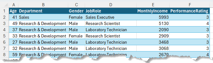
PivotTables also require your data to be formatted in a tabular format where there is a separate column for each field, like the example below:

Use Power Query to unpivot your data if required.

Accessing the Grouping Feature in Excel

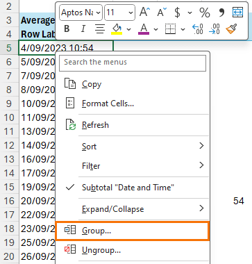
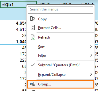
To access the grouping feature: Right-click an item in the field you wish to group > Select 'Group' from the menu:

Group Dates and Time

With PivotTable grouping we can quickly sum monthly data into quarterly and yearly summaries, and easily segment time-based data into specific time intervals.

For example, accountants often need to summarize monthly data into quarters or years, and Grouping by Days of the Week enables retail and service industries to analyze data based on specific days.

Grouping Numbers into Intervals or Bands

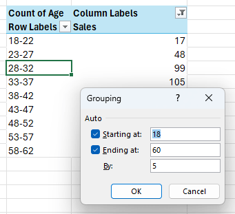
We can easily create numeric intervals, for example, group sales or other numbers into defined ranges like 1-10, 11-20, etc.

And segment data into bands: for instance, classify customers into bands based on their purchase amounts. Or employees into age bands as shown here:

 

Custom Groups

Want to group data that doesn't fit traditional categories? Create your custom groups to tailor your analysis to your needs.For example, you can group specific row/column labels together, which is especially useful for categorical data.

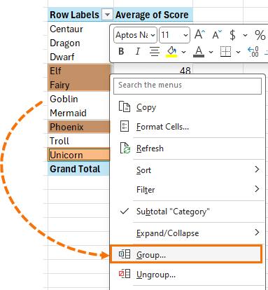
To create a custom group, select the items you want to group > right-click > Group:

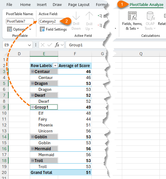
The new group has the default name: Group1.

Rename it by typing over the text in the cell (E9) and then give the field a new name via the PivotTable Analyse tab:

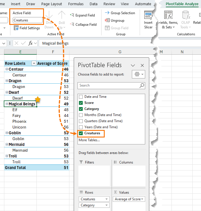
This adds a new field to the PivotTable which I’ve renamed: ‘Creatures’ and you can see in the image below that it appears as a new field in the field list.

I’ve also renamed Group1, ‘Magical Beings’ by typing over ‘Group1’ in PivotTable cell E9.

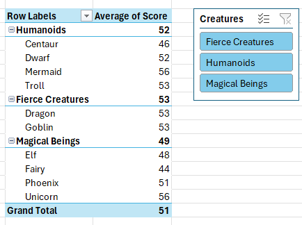
Continue adding groups as required. And because this is now a new field, I can add a Slicer for it:

Custom Group Gotchas: any other PivotTables based on the same source data (that share the pivot cache) will also have these custom groups added, but they won’t pick up the group names you manually type into the cells of the PivotTable.

You will need to repeat the name labels for each PivotTable individually or copy the one you’ve changed and rebuild the others.

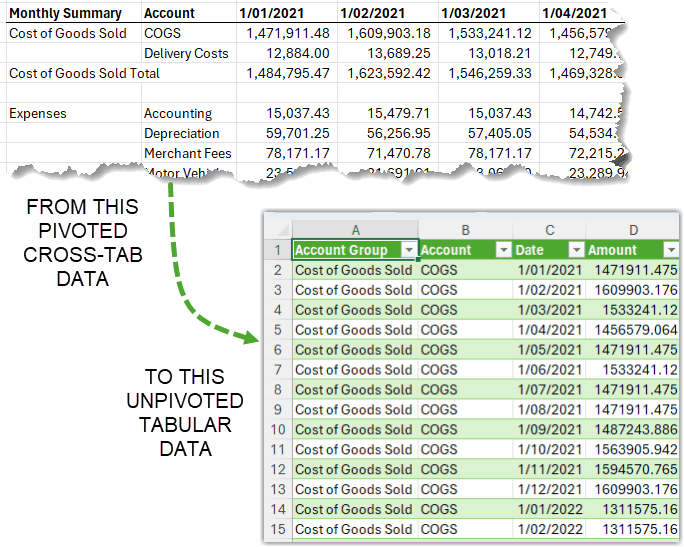
Grouping Cross-tabular Data

Accountants in particular love working with cross-tabular data, like the example below where the dates run across the columns and the items or categories listed down the rows.

Watch this video to see the problems you’ll encounter when you try to Pivot data in this format. Spoiler, it’s a train wreck.

To fix this, first we need to unpivot the data using Power Query, as shown in the video at the top of this page.

We can then build a PivotTable that groups the data by quarters and Item, and sums the Amount column:

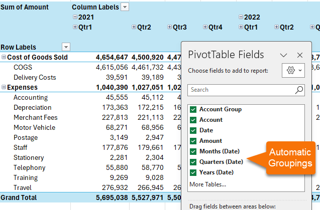
When working with dates in PivotTables, Excel will automatically group them when they’re used in row or column labels.

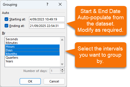
To modify the default grouping, right-click on the date field in the PivotTable > Group:

In the Grouping dialog box, choose the groups you want:

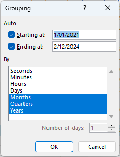
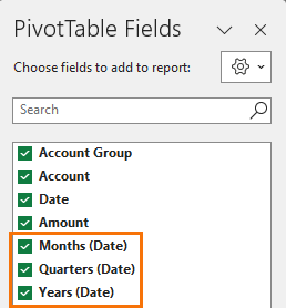
Tip: if your data spans multiple years, include ‘Years’ in the grouping.

You’ll see these fields are added to the PivotTable field list for use in your reports:

PivotTable Grouping Limitations

PivotTable grouping in Excel offers powerful capabilities, but it does come with certain restrictions and considerations:

1. Blank Cells: If there are any blank cells in the column you're trying to group, Excel will throw an error. You'll need to either fill or remove blank cells before grouping.
2. Mixed Data Types: Grouping won't work if your column has mixed data types, such as a combination of text and numbers.
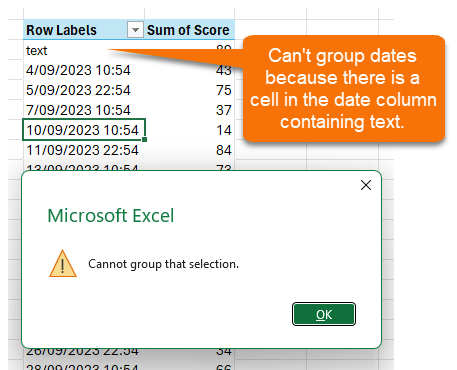
3. Date Grouping: When grouping by dates, the data must be valid date serial numbers. If there are invalid dates or non-date entries like text, the grouping will fail.

   

4. Grouping Shared Field: If you group a field in one PivotTable, and if that field is also present in another PivotTable, the second table will also get grouped. This happens because both PivotTables share the same pivot cache.
5. Manual Groups: If you're creating manual or custom groups, you can't use the usual calculated field or item capabilities in PivotTables and will see an error like this:

   

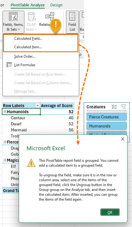
If you need calculated fields and items in your PivotTable and you get this error, then add a field to your source data that enables you to group the data the way you want without having to use the PivotTable Grouping tool. e.g. if you want to group your dates by month, add a Month column to the source data.

6. Grouping on External Data: Depending on the source of external data, you might encounter limitations or extra steps when trying to group data. For instance, when connecting to OLAP sources, the grouping has to be defined in the cube itself and not in the Excel PivotTable.

Next time you need to summarize data into groups, instead of doing it the hard way with formulas, use PivotTable grouping to make your life easier.

Get started with PivotTables with my Excel PivotTable Quick Start course.