Is it possible to use conditional formatting in the row labels for a text value that will highlight the entire row across for all values? I have 64 different text values that I would like to highlight all of its values across the pivot table. The attachment is just a small sampling of the data I'm utilizing.
I also didn't know if there was an easier way to create a conditional formatting rule to highlight cells containing text when I have a range of 64 text values. Or would I need to add each different text value as its own rule?
Appreciate any help on this.
Theresa Diers
Hello Theresa,
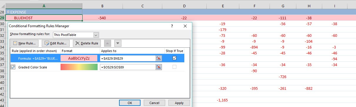
To highlight the entire row you will need to add a Conditional Format based on a Formula.
The formula will look like this:
=$A$29="TEXT"
Then in the Applies To section you need to highlight all the cell's in the row that you want to apply this format to. Hit Apply.
Unfortunately you will have to create this for each of the text values 🙁