Hi,
In the attachment - there is column A.
I want it to focus on the rows of the number 9607 from column B.
And will display the numbers from column A in one cell with commas in between
As in the file - in the example in cell D3
And I need him to do this to me for every other number from column B.
So that the end result will be the same as in cells A10: B11.
(If impossible with commas then - sixty each number in a separate cell -
As in file in cells D1: G1)
Thank you so much for the help !!
Leah

Bring your data into a Data Model and write a measure to consolidate the data separated by commas. See my attached file.
A tutorial on this is at: https://sfmagazine.com/post-entry/july-2018-excel-reporting-text-in-a-pivot-table/
Seems like an ingenious idea !!!
If you can attach the file - it was not attached in a previous post
It will help me a lot !!!
Thank you!!!!!
Sorry about the attachment. Attached now.
Thank you!
Honestly, I had a hard time understanding how to do it ...
I want to enter on the file you brought me the data
Then go to Pivot and click Refresh
The problem is that the information table is not dynamic so it does not update me
So if it is not difficult for you to set the original table to be dynamic
And so I can use with the file.
Thank you Thank you Thank you!!!!!!!!!
Leah
Highlight your table and click on Add to Data Model and click on refresh all. Same as you would in a regular Pivot Table. Make sure you are in Power Pivot.
The truth is, I do not know Power Pivot
That's why you ask such simple questions,
But Suri ... it does not work for me
I took your table, switched to a Power Pivot card, marked the table, clicked Add to data model, Power Pivot opened for me, where - Issue 1 - was updated but RANGE's issue was not updated - so when I returned to Excel I clicked Refresh everything - failed.
How do I also update the RANGE issue?
Thank you so much for your patience for my questions !!!!
Leah
Here is what Microsoft suggests

Hi Lea,
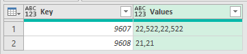
You can use Power Query to do this, see the attached file.
These are the steps:
1. Create a table from your data (CTRL+T)
2. Set the Values column to text
3. Group the data by the Key column (9607, 9608 etc)
4. Use Text.Combine to concatenate the Values together with a comma separator
Here's the query
let
Source = Excel.CurrentWorkbook(){[Name="Table1"]}[Content],
#"Changed Type" = Table.TransformColumnTypes(Source,{{"Value", type text}}),
#"Grouped Rows" = Table.Group(#"Changed Type", {"Key"}, {{"Vals", each _, type table [Value=nullable text, Key=number]}}),
#"Added Custom" = Table.AddColumn(#"Grouped Rows", "Values", each Text.Combine([Vals][Value] ,",")),
#"Removed Columns" = Table.RemoveColumns(#"Added Custom",{"Vals"})
in
#"Removed Columns"
Giving this
If you want to learn Power Query or Power Pivot we have courses for both
Regards
Phil
