Hi,
Need some advice. I need to create a spreadsheet in where in sheet 1 once I put the text in column A2, it will search if this name is available or present in sheet 2.
I need to use the first four characters of the name in col. A2 to find some matches in sheet 2 and it will give the results horizontally.
Example: the data that I have inputted in sheet 1 A2 is Eastman, Results will appear in B2, C2, D2 and so on.
Name(a2) Result1(b2) Result2(c3) Result3(d4)
Eastman Eastway Eastwest Eastman
Once wondering what formula to use in this.
Thanks for the help.
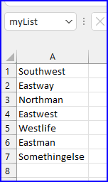
Provided you are on Excel for MS365 or 2021, you can use TRANSPOSE and FILTER. Let's say the list of keywords in Sheet2 is in a named range called "myList", the following formula in B2 will produce what you ask for.
=TRANSPOSE(FILTER(myList,LEFT(myList,4)=LEFT(A2,4)))


Thanks for this.
I tried using this formula but says function is not valid. Was wondering if you can attach the sample excel so I can look at it?
Hi,
it seems the filter is not working as it says function not valid. Is there a simple vlookup function instead?
Sorry to have missed your original answer. Attaching the file I used in my example. Not that it doesn't work if you don't have Excel for MS365 or 2021.
No worries and thanks.
I tried changing the text in A2 but suddenly the formulas in B2-D2 became #Name. Even copying the formula on the next row results to that error.
Hello,
I have borrowed the sample file that Riny uploaded, added two helper columns and use the first helper column to find matching data.
See attached file for an example.
Br,
Anders
