Hello all!
Long story short, I am able to conditional format a range to highlight every other group in an unfiltered range. But I am having a hard time doing it for a filtered range.
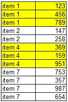
For example. For the filtered range below, I want item 1 and item 4 highlighted.

Thanks in advance!
If I understand you correctly you want to be able to always highlight alternating groups in a table. Filtered or unfiltered.
Thus, when you filter out Item 4, then Items 1 and 7 should be formatted.
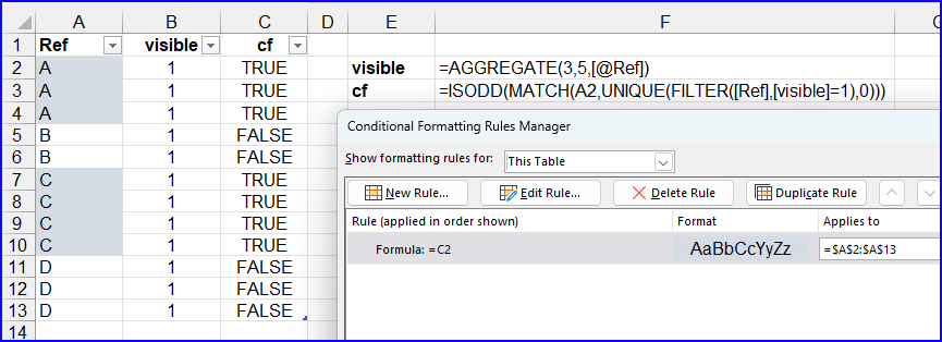
Perhaps there's another way but I came up with one that requires two helper columns that may be hidden.
One that determines if the row is visible or not and another that sets TRUE or FALSE that will be the basis for the conditional formatting rule. See if you can get this implemented in your own schedule, provided my assumptions were correct of course!

See attached.
Edit: In order to use consistent structured table references, the formula in the cf column should actually be
=ISODD(MATCH([@Ref],UNIQUE(FILTER([Ref],[visible]=1),0)))
This is great! Works great with a table range. Any idea on how to do this for a spilled range? Aggregate doesn't seem to like spilled ranges 🙁
I'm using a spilled range because the rows of data isn't always the same. I "could" put a macro to add or delete rows, but rather make it dynamic and based on the data.
Thanks again! If all else fails, I'm gonna use this.
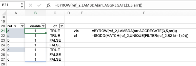
Ah, I see. If your Excel version supports LAMBDA (and helper functions), you can put AGGREGATE in a BYROW/LAMBDA function to make it spill as demonstrated in the picture.

