Hello all. I've been digging all around the cloud for this, and it's tough to type in a concise search phrase, so hopefully someone can help me.
I have a worksheet with multiple tabs. One of my tabs is the main (destination) Report for my data. I also have secondary tab with a list of Retailers, including columns for Address, City, State, Zip (as headers of a Table).
I created a dropdown list in my Primary sheet/tab for the names of each retailer. I have matching headers on the Primary sheet as the Secondary sheet (Table).
My goal is to choose the name of the Retailer, and then each corresponding cell in that row (under each matching header of the table for that Retailer) to automatically populate in the same cells of the Primary sheet.
In case I'm not articulating this correctly. I want to choose "Great Lakes Ace" from the dropdown in my Primary sheet, and then the cell values to reference the Table in my secondary sheet, and pull the Street Address, City, State, and Zip for that Retailer.
I tried some IF/THEN formulas, but could only get it to work for one retailer at a time. Also, I believe you can only nest so many and retailer list is at 25+ and will continue to grow.
Any guidance here would be greatly appreciated. Thanks.
Hi Jimmy,
Do you have a workbook with sample data we can see?
Regards
Phil
Yes, a workbook would be helpful, but you can probably just use VLOOKUP or Index/Match to get what you want.
Thanks all. Sorry, I understand the spreadsheet itself would be helpful. However, oddly enough, I tried to attach it and this platform gave me an error that it's too large (even though there's barely any data right now).
So I'll try to upload some screenshots for reference... I appreciate any insight. Honestly, I am quite an amateur, though I have figured a few data validation formulas myself thus far. Hopefully this is child's play for you...
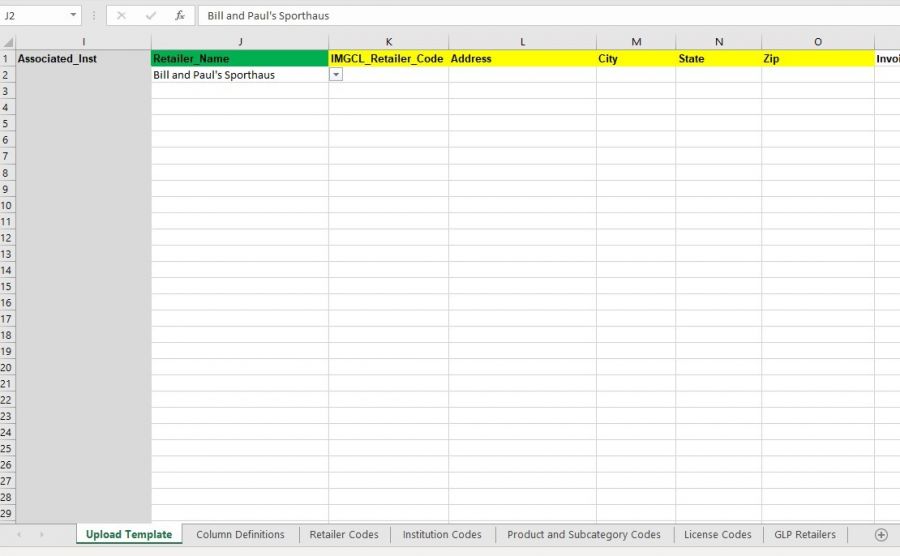
The first screenshot is my Primary sheet, where I would be choosing a retailer from the dropdown I created, and then ideally columns K, L, M, N, O will populate based on values from columns B, C, D, E, F from my Table in screenshot two (Tab "GLP Retailers).
I think this is a straightforward description. But please feel free to hit me with any follow up questions.
I really appreciate it.
-JA
![]()
Jimmy's workbook is attached below.
First, I would put the data on the first sheet in a table (like it is in your last sheet). In fact, I would put everything I possibly could in tables as they offer great advantages.
I added Index/Match formulas in the columns for the retailers address so they will populate automatically. In a table, the formula automatically is added to all rows in a table, but you can copy down the formulas as far as you need to if you'd like.
Hi gents. Thanks for the insight/advice here. I added the Index/Match function and it works! There's just one follow up: I cannot drag down the formula to subsequent rows without so many cell numbers moving up sequentially. Is there a way I can scale this formula downward per column (K,L,M,N,O) where the reference value cell (Here it's Row J) stays static, but my Index + Match value ranges (for the table) stay the same?
Is this what you meant by "In a table, the formula automatically is added to all rows in a table"?
Thanks so much.
Hi again gents. I am 99% of the way there. I started to create this report, but I have an issue with scaling these Index/Match formulas downward in Columns K, L, M, N, O. Some are pulling the incorrect address from the Retailer chosen in the dropdown. Some are not pulling any Data at all. Can you help? I will try to upload the current sheet as-is, and if it doesn't work, I'll ask Phil to re-upload it to the thread manually. Any help is appreciated. Thanks!
I've uploaded a file where I put the data in the first sheet in a table. I don't know if you want all the data in the same table, but you should get the idea. As you start typing in the first empty row below the last row of the table, it will automatically expand, and the formulas will copy down automatically.
I'm sorry, I don't see an attachment to your latest response.
I think I know what happened. The file was too big and was rejected. I deleted a lot of rows on your "Retailer Codes" tab so the size could be reduced enough to be able to upload it. Are you able to see it now?
Hello,
The problem you have is due to not locking the lookup range.
In cell K3 you have this formula: =INDEX('GLP Retailers'!B4:B100,MATCH(J3,'GLP Retailers'!A4:A100,0))
In cell K4 you have this formula: =INDEX('GLP Retailers'!B5:B101,MATCH(J4,'GLP Retailers'!A5:A101,0))
In cell K8 you have this formula: =INDEX('GLP Retailers'!B4:B105,MATCH(J8,'GLP Retailers'!A9:A105,0))
As you notice the lookup range differs. Lock the cell ranges before you copy down and to the right.
In cell K2 write the formula like this: =INDEX('GLP Retailers'!B$4:B$100,MATCH($J2,'GLP Retailers'!$A$4:$A$100,0))
Or use table references: =INDEX(Table1[IMGCL_Retailer_Code],MATCH($J2,Table1[[Retailer_Name]:[Retailer_Name]],0))
Or use VLOOKUP: =VLOOKUP(Table2[@[Retailer_Name]:[Retailer_Name]],Table1,2,0) Just remember to change the column reference 2 when copying to the right.
@Greg - I still was unable to see any attachments. In the meantime, I think this is solved, and I really appreciate your help.
@Anders. Thanks so much for your insight here. I chose to go with the VLOOKUP process, and it has worked out nicely. Thanks so much everyone for your help with this. I learned a lot!
Hello Jimmy,
Great that it works fine for you now.
