Hi Humayun,

This is what you are looking for

https://www.myonlinetraininghub.com/excel-data-validation-with-dependent-lists

 

these posts will also help 

https://www.myonlinetraininghub.com/excel-dependent-data-validation

https://www.myonlinetraininghub.com/excel-factor-19-dynamic-dependent-data-validation

 

Regards

Phil

Hi Phil,

First of all thanks for the reply.

I have gone through the links and some similar methods in the past. The problem is that the source data which I have is in a tabular format (not sure if I am using the correct term) whereas the source data there in the links is a bit different.

There Data

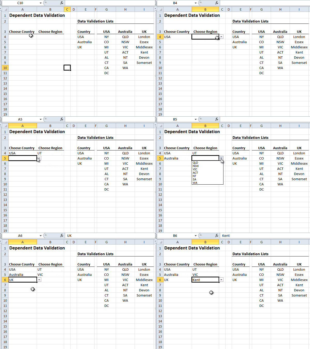
Parent list in one column and then all the countries will be treated as headings besides the parent column and under those headings will be the child data and so they can use the indirect function. Have a look at the image below.

 

 

 

 

 

My Data (All in one place in Sheet 1)

REF # - ARTICLE NAME - SIZE
414 .....DUVET ..............135 X 200 CM
414 .....DUVET................140 X 200 CM
415 .....DUVET ...............150 X 200 CM
415 .....DUVET ................160 X 200 CM
416...... PILLOW ...............70 X 80 CM
416 ......PILLOW ...............80 X 80 CM
417.......DUVET ...............90 X 80 CM
417 ......PILLOW ...............100 X 80 CM
417 ......PILLOW ................60 X 40 CM

 

Now in sheet 2 when I enter a ref # in cell A2 a dependent drop down (dependent on the data entered in cell A2) list appear in cell B2

For Example

If I enter 414 in A2 > list will appear showing only DUVET

If I enter 417 in A2 > list will appear showing DUVET & PILLOW

Here is the formula I am using in Data Validation

=OFFSET(Sheet1!$B$1,MATCH(A2,ref,0),0,COUNTIF(ref,A2),1)

 

Required

Now all I want is another formula for cell C2 (in data validation) which shall give a drop down list which would be dependent on values of cell A2 & B2

For Example

If I enter 414 in A2 & select DUVET from the dependent drop down list in B2 > then a list should appear in cell C2 showing 135x200 CM & 140x200 CM 

If I enter 417 in A2 & select DUVET from the dependent drop down list in B2 > then a list should appear in cell C2 showing only 90x80 CM

 

Its this formula

=OFFSET(Sheet1!$B$1,MATCH(A2,ref,0),0,COUNTIF(ref,A2),1)

which needs to be modified for the list I want in C2 ( which will be dependent on both entries of A2 & B2)

 I am unable to do it - tried a lot though 🙁

Regards,

Humayun

Hello Humayun,

Please share a sample file showing your data structure.

Have you checked this info?

Hi Anders,

Thanks for the reply.

I will look into the link you provided and also I will share a sample file tomorrow as today I won’t be having access to my computer.

Regards,

Humayun