From time to time I get asked the question “what order do formulas evaluate?”
The acronym BEDMAS can help you remember. It stands for:
Brackets: Any operation(s) contained in brackets will be carried out first followed by any exponents.
Exponents: Then any exponents like ^ or SQRT
Division or Multiplication (left to right): Excel considers these to be of equal importance, and carries out these operations in the order they occur from left to right in the equation.
Addition or Subtraction: The same goes for addition and subtraction. They are considered equal in the order of operations. Whichever one appears first in an equation, either addition or subtraction, is the operation carried out first.
Ok, so what if you know all that (after all you probably learnt BEDMAS at school way-back-when) but you’re still stuck because your formula isn’t returning the result you want.
Well, thankfully Excel has a tool for that too.
Evaluate Formula Tool
The Evaluate Formula tool allows us to see how each component of a formula evaluates, one step at a time.
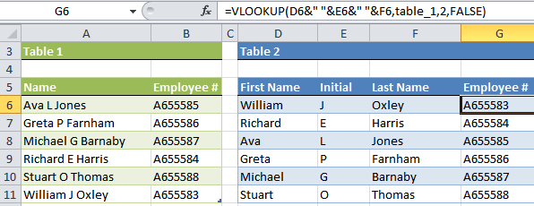
Let’s take the VLOOKUP formula we looked at last week as an example:
How to use the Evaluate Formula Tool
- Select the cell containing the formula you want to evaluate. Ours is in G6.
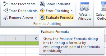
- On the Formulas tab of the Ribbon in the Formula Auditing group select Evaluate Formula.
The Evaluate Formula dialog box will open:
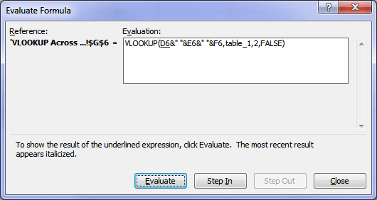
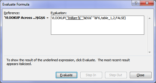
- Click the ‘Evaluate’ button to view the value of the underlined reference. In the example above the underlined reference is cell D6, and you can see below it evaluates to ‘William’.
- If the underlined reference is part of another formula you can use the ‘Step In’ button to display the other formula. Then ‘Step Out’ to go back and continue evaluating.
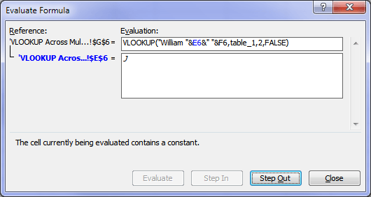
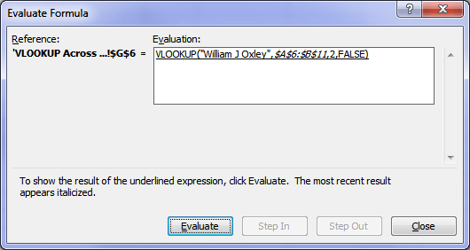
- In the image below you can see all but the last step of the formula evaluated:
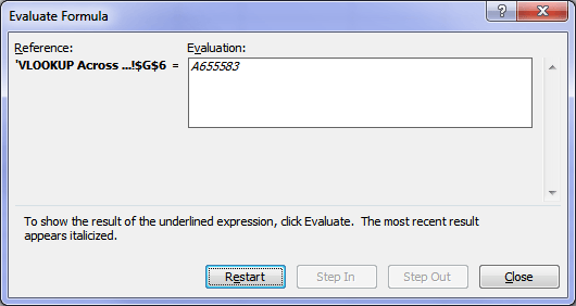
- And finally the result:
The Evaluate Formula tool is especially useful for nested formulas that may not be returning the correct result.
I also like to use it to find why I’m getting # errors or checking that the result is calculating as I expect.
But be warned; it can’t work miracles. If you can’t get Excel to even accept your formula then you may need to consult your office Guru first 🙂
FILTER(‘Finance Tec Competency’!E:E, ISNUMBER(MATCH(‘Finance Tec Competency’!C:C, ‘Finance Tec Competency’!CA$12, 0)))
I want to drag down the above formula but I want to change Finance Tec Competency’!E:E to be Finance Tec Competency’!F:F “””auto”” HOW??
You can’t drag it down because you have whole column references E:E etc. You could drag it across, but I would strongly recommend you replace the whole column references with the actual range + some spare rows to allow for growth or put your source data in an Excel Table. While some Excel functions can now ignore empty cells in whole column references, not all can and sometimes even those that can don’t under certain conditions, so I always avoid them.
If you’re still stuck, please post your question on our Excel forum where you can also upload a sample file and we can help you further.
Question:
I tried to create a formula to do a Match on two separate columns. This is because we have the same servers (same IP) but different vulnerabilities (Plugin IDs) for them.
This is my formula:
=IF(MATCH(A2,’Existing – Server Application’!$A$2:$A$412,0),AND(MATCH(G2,’Existing – Server Application’!$H$2:$H$412)),”False”)
I get an #N/A error and can’t seem to get around it. What I need is: If cell A2 of “Worksheet 1” matches anything in Column A of “Worksheet 2” and cell G2 of “Worksheet 1” matches same in Column H of “Worksheet 2” then return a True, otherwise False.
Hi Adam,
Please post your question on our Excel forum where you can also upload a sample file and we can help you further.
Mynda
Formula Not Working … Please Help …
=IF(
LeadCount!$B5 = “All” ,
IF(
LeadCount!D$2 = “All” ,
SUM(
COUNTIF(
USA!$D:$D,
”Interested”
),
COUNTIF(
USA!$D:$D,
”Forwarded the documents”
),
COUNTIF(
USA!$D:$D,
”Will visit office”
)
) ,
COUNTIF(
USA!$D:$D,
LeadCount!D$2
)
) ,
IF(
LeadCount!D$2 = “All” ,
SUM(
COUNTIFS(
USA!$D:$D,
”Interested”,
USA!$Z:$Z,
LeadCount!$B5
),
COUNTIFS(
USA!$D:$D,
”Forwarded the documents”,
USA!$Z:$Z,
LeadCount!$B5
),
COUNTIFS(
USA!$D:$D,
”Will visit office”,
USA!$Z:$Z,
LeadCount!$B5
)
) ,
COUNTIFS(
USA!$D:$D,
LeadCount!D$2,
USA!$Z:$Z,
LeadCount!$B5
)
)
)
Hi Vishal,
It’s very difficult to troubleshoot a formula like this without the file. Please post your question on our Excel forum where you can also upload a sample file and we can help you further.
Mynda
=(IF(F9>=25,”Critical”), (F9>=20,”High”), (F9>=15,”Medium”,”Low”)))
This formula is not working
Try this:
=IF(F9>=25,”Critical”, IF(F9>=20,”High”, IF(F9>=15,”Medium”,”Low”)))
Mynda
Please check this formula. =IF(AND(AP24>0,AQ24>0,AH24>0),”BUY CE”,IF(AND(AP24<0,AQ24<0,AH240,AQ4<0,AH24<0),"BUY PE",IF(AND(AP0,AH24>0),”BUY PE”,IF(AND(AP24>0,AQ24>0,AH24<0),"BUY PE")))))
I want to make it happens for all the three AP24,AQ24,AH24. now its considering only AP24 and AQ24.
Hi Khem, please post your question on our Excel forum where you can also upload a sample file and we can help you further.
Could you please check these three formulas?
=ARRAYFORMULA(IF(ISBLANK(F2:F),,”S”&Input!$B$1&VLOOKUP(F2:F,’New DRCP Verlauf’!C:P,14,0)&”A”&TEXT(VLOOKUP(F2:F,’New DRCP Verlauf’!C:P,16,0),”0000″)))
=ARRAYFORMULA(IF(ISBLANK(F2:F),,VLOOKUP(F2:F,’New DRCP Verlauf’!C:P,18,0)))
=ARRAYFORMULA(IF(ISBLANK(F2:F),,”S”&Input!$B$1&VLOOKUP(F2:F,’New DRCP Verlauf’!C:P,14,0)&”A”&TEXT(VLOOKUP(F2:F,’New DRCP Verlauf’!C:P,16,0),”@”)))
Hi Rohan,
There’s no such function as ARRAYFORMULA in Excel.
Mynda
=IF(OR(F4=”EID-UL-FITAR”,F4=”EID-UL-AJAHA”,[@RELO]=”M”,CODE!F5*1,IF(Sheet1!D7>=”H”,F4=”DURGA PUJA”,F4>=”BUDDHA PURNIMA”,CODE!F5*1,IF(F4>=”MONTH BILL”,,CODE!F5*1,””))))
Yes
Please correct this formula.
=LOOKUP([@Parent],Table37[[Parent]:[Name]],Table37[Name], OR(LOOKUP([@Parent],Table1[[ID]:[Title]],Table1[Title])
I get “The formula is missing an openeing or closing parenthesis” error.
Hi Grant, you can’t structure the formula like that with OR at the end. Please post your question on our Excel forum where you can also upload a sample file and we can help you further.
please correct
=IF(AND(B1,C1,D1,E1)=1,”nedovoljan”,IF(AND(G1=3.5),”vrlodobar”,IF(AND(G1=2.5),”dobar”,IF(AND(G1=1.5),”dovoljan”,IF(AND(G1<1.5),"nedovoljan","nedovoljan")))))
Hi Kenima,
Each AND argument must be a logical test. You can’t list all cells and then only 1 logical text i.e.:
You also don’t need AND for the remaining IFs because there is only one condition:
Mynda
=IF(OR(E5=”In House”,KN5>=15,E5=”Outside”,KN5>=25),”Sufficient stock”,”Near to Nill”)
please correct
Hi Naveed,
What is wrong?
Or, how do you want it to work, if it’s not working as expected?
=IF(AND(D7>0,H7>0),”FRESH LONG”,IF(D7<0,H70,H7<0),"FRESH SHORT",IF(AND(D70),”SHORT COVERING”,”)
THIS SYNTAX WONT WORK ,KINDLY RECTIFY THIS FORMULA
Try:
=IF(AND(D7>0,H7>0),"FRESH LONG",IF(AND(D7<0,H7<0),"FRESH 14:14",IF(AND(D7>0),"SHORT COVERING","No Match")))
Make sure you put the logical conditions needed for each nested IF function.
=IF(AND(D2=K2,”Q1 2022″,IF(D2=H2,”Q2 2022″,IF(D2=I2,”Q3 2022″,IF(D2=J2,”Q4 2022″,””))
Please help me correcting this
Hi Anup,
You haven’t used AND correctly. Try:
However, a more efficient way to write this formula is explained in this IF Function video tutorial.
Mynda
=IF(H3>=50,”Pass”,”Fail”),IF(M3>=1,”Repeat”)
pls send me correct one
=IF(M3>1,”Repeat”,IF(H3>=50,”Pass”,”Fail”))
IF(AND(S2=((“Priority 4”,U2<=2), "Met","Not Met"),(("Priority 5",U2<=7),"Met","Not Met")))
I am not getting the answer
try:
=IF(AND(S2=“Priority 4”,U2<=2), "Met",IF(AND(S2="Priority 5",U2<=7),"Met","Not Met"))
How to write formula in excel : 25% of quantity or Rs.5000 whichever is greater
Hi,
Try:
=MAX(5000,A1*0.25)
Where is my mistakes here in this? this formula excel not excepting. looking your urgent reply please.
=IF(I3=-26,”infinity”,IF(I3=-25,”infinity”,IF(I3=-24,”infinity”),IF(I3=-23,”infinity”),IF(I3=-22,”infinity”),IF(I3=-21,”infinity”),IF(I3=-20,”5.49″),IF(I3=-19,”5″),IF(I3=-18,”3.47″),IF(I3=-17,”4″),IF(I3=-16,”6.84″),IF(I3=-15,”2.24″),IF(I3=-14,”3.53″),IF(I3=-13,”3.23″),IF(I3=-12,”3.23″),IF(I3=-11,”2.93″),IF(I3=-10,”3.2″),IF(I3=-9,”2.65″),IF(I3=-8,”2.38″),IF(I3=-7,”2.53″),IF(I3=-6,”2.62″),IF(I3=-5,”2.46″),IF(I3=-4,”2.48″),IF(I3=-3,”2.26″),IF(I3=-2,”2.2″),IF(I3=-1,”2.26″),IF(I3=0,”2.19″),IF(I3=1,”2.1″),IF(I3=2,”2.02″),IF(I3=3,”2.01″),IF(I3=4,”1.8″),IF(I3=5,”1.94″),IF(I3=6,”2.06″),IF(I3=7,”1.76″),IF(I3=8,”1.76″),IF(I3=9,”1.74″),IF(I3=10,”1.79″),IF(I3=11,”1.59″),IF(I3=12,”1.57″),IF(I3=13,”1.65″),IF(I3=14,”1.54″),IF(I3=15,”1.76″),IF(I3=16,”1.36″),IF(I3=17,”1.49″),IF(I3=18,”1.13″),IF(I3=19,”1.62″),IF(I3=20,”1.2″),IF(I3=21,”1″),IF(I3=22,”2″),IF(I3=23,”1″),IF(I3=24,”1″),IF(I3=25,”1″),IF(I3=26,”1″),IF(I3=27,”1″)))
Hi Tanvir,
You should setup a table with 2 columns with your parameters, it’s not a good idea to use so many nested functions.
With a lookup table, the formula is much simpler: =INDEX(Table1[Result],MATCH(I2,Table1[Value],0))
In your formula, as an example:
=IF(I3=-26,”infinity”,IF(I3=-25,”infinity”,IF(I3=-24,”infinity”),IF(I3=-23,…
there should not be a closing paranthesis before the last IF in this example, all closing paranthesis should be at the end of the formula.
Some older excel versions will not accept too many nested IF’s, you should go for a lookup table.
if B having annual target 230917 to find monthly target and find if a month having 20 day to calculate per day target
Hi Uma,
Daily target should simply be: =B1/12/20
Please correct my formula =COUNTIFS(DIS!B:B,{“Taimani”,”chaman”,”Khushalkhan”},DIS!E:E,{“Group Loan”,”GMRB”})
Try:
=COUNTIFS(DIS!B:B,”Taimani”,DIS!B:B,”chaman”,DIS!B:B,”Khushalkhan”,DIS!E:E,”Group Loan”,DIS!E:E,”GMRB”)
=IF(AND(B4>=80,C4>=80,D4>=200),”Passed all”,IF(AND(B4=80,D4=80,C4<80,D4<80),"Passed Science only",IF(AND(B4<80,C4=200),”Passed TOEFL only”,IF(AND(B4>=80,C4>=80,D4<200),"Passed both English and Science",IF(AND(B4=80,D4>=200),”Passed both English and TOEFL”,IF(AND(B4>=80,C4=200),”Passed both Science and TOEFL”))
Did you have a question, Lina?
Hello,
i think there is something wrong with this formular but i can not identify whats wrong.
=IF($A$5:$A2489=””,””,IF(COUNTIF(‘Scanned Assets’!$A$2:$A2428,$A$5:$A2489)>0,”Y”,”N”))
I have about 2000 asset numbers, but the formular is only reading against 950 cells, so any number after cell 950 is not recognized.
Basically what i am trying to do is – Already have the assets numbers, I want a Y once i scan assets and the number is part of the numbers i already have.
Please can you help?
Hi Dero,
The first argument of the IF formula should only reference one cell, not a range of cells. That said, I don’t think the COUNTIF will be doing what you want either. Please post your question and Excel file on our forum where we can help you further.
Mynda
=IFERROR(1-(SUM(IF(D13:D62={“CLI / ANCILLARY”,”ENDOSCOPY”,EMERGENCY ROOM”,”IV THERAPY”,”OB OUTPATIENT”,OBSERVATION”,”RECURRING”,SAME DAY SURGERY”,”WOUND HEALING CLINIC”},H13:H62,0))/SUM(COUNTIF(D13:D62,{“CLI / ANCILLARY”,”ENDOSCOPY”,”EMERGENCY ROOM”,”IV THERAPY”,”OB OUTPATIENT”,”RECURRING”,”SAME DAY SURGERY”,”WOUND HEALING CLINIC”}))),”%”)
I keep getting an error message at D13:D62 I’m sure there’s plenty more none of my sheet with the exception of two columns will populate a % I want. If there is a time I can screenshare and someone help me I’ll of course happily pay for the time. Here is one of 48 other percntages in the same sheet I cannot get to work 🙁
Hi Tiff,
Can you upload to our forum a sample of your data, with a manual example of expected results?
Does not seem like a complicate problem, but we need to see some data to test the formulas.
Catalin
Uploading now
=IF(FIND(“@nscglobal”,[Created by]),”Yes”,IF(FIND(“@axiomtechnologies.com”,[Created by]),”Yes”,IF(FIND(“@se.relacom.com”,[Created by]),”Yes”,IF(FIND(“@DaisyGroup.com”,[Created by]),”Yes”,IF(FIND(“@ecfix.com”,[Created by]),”Yes”,IF(FIND(“@dynacons.com”,[Created by]),”Yes”,”NO”))))))
What’s wrong with this?
Hi Glenn,
The logical test in the IF function expects a boolean data type. FIND(“@nscglobal”,[Created by]) will return 2 different data types: N/A (error), when that text is not found, and a positive number if that text is found. In other words, errors are not handled. Make sure your formula returns the expected data type, use this for example: =ISNUMBER(FIND(“@nscglobal”,[Created by])) instead of FIND(“@nscglobal”,[Created by]). ISNUMBER will return TRUE/FALSE, no matter if FIND function fails.
=IF(D13=12%,IF(AND(D15>=0%,D15=26%,D15=46%,D15=61%,D15=81%,D15=0%,D15=26%,D15=46%,D15=61%,D15=81%,D15=0%,D15=26%,D15=46%,D15=61%,D15=81%,D15=0%,D15=26%,D15=46%,D15=61%,D15=81%,D15=0%,D15=26%,D15=46%,D15=61%,D15=81%,D15<=100%),"4%")))))))))))))))))))))))))))
Hi Khalil,
What is your question?
Regards
Phil
‘=if(C15=’Tax Not Included’,0,if(and(C15=’Tax on Material Only’,sum(E12:E13)*D15),if(and(C15=’Tax on Labor Only’,sum(E3:E11)*D15,if(and(C15=’Tax on Labor &Material’,sum(E3:E13)*D15))))
Can’t get this to work. Can anyone tell me what is wrong with this?
Hi Joe,
Try wrapping your text in double quotes instead of single quotes. e.g.
Mynda
Hi Mynda,
I frequently use the evaluate formula tool however I cannot resize the evaluate formula tool window. This makes evaluating array formulas particularly hard. Do you know of an evaluate formula add-in with a larger formula evaluation screen or perhaps a way to expand the evaluate formula tool window?
-Chris
Hi Chris,
This is a gripe of us MVPs too. Unfortunately it and many other dialog boxes cannot be resized 🙁
That doesn’t mean we don’t keep asking at every Microsoft Summit when we meet with the Excel developers.
Mynda
Can anybody help detecting problem in following formula:
(every time i pressed enter, the result shown:#NAME)
=IF(And(D2=”Dhaka”,F2<5000),F2*70%””, IF(And(D2=”Rajshahi”,F2<5000),F2*65%””, IF(And(D2=”Feni”,F2=10000),F2*60%””, IF(And(D2=”Rajshahi”,F2>=10000),F2*55%””, IF(And(D2=”Feni”,F2>=10000),F2*50%””))))))
Any Syntax Error?
Hi Umar,
The double quotes after the % signs shouldn’t be there e.g. F2*70%””
But without seeing the file it’s hard to say otherwise. You’re welcome to post your question and Excel file on our forum where we can help you further.
Mynda
IF(((AJ3+AK3+AL3+AM3+AN3+AO3)/6)*70>=70,”70″, “(AJ2+AK2+AL2+AM2+AN2+AO2)/6)*70”)
This is the formula that I am using. I am adding values to figure out a students grade out of 70 without letting the value exceed 70. That is working, I can not get it to use the second formula if it doesn’t exceed 70. Help please.
Hi Brandon,
Looks like too many double quotes. Try this:
Double quotes return/specify text.
Mynda
Something to remember from our Highschool days.
Here’s a question for you, is there anyway to tell from the error that excel returns (#Name, #Value) as to what might be wrong?
Hi Bobcat,
Yes, you can tell from the error what might be wrong. I haven’t written a list of them but you can find one at the link below (see the right hand side of the page under ‘See also’):
https://office.microsoft.com/en-us/excel-help/correct-common-errors-in-formulas-HA010066323.aspx
I should add writing about that to my To-Do list 🙂
Kind regards,
Mynda.