New Excel Functions for Accountants

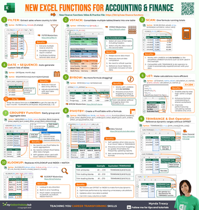
Microsoft has recently released a set of game-changing Excel functions that would’ve been a dream come true back in my accounting days. These functions will make your work easier, faster, and (dare I say) even a little bit fun.

I’ll reveal my favourite function along the way, but I’d love to know which one clicks for you. Leave a comment below - and don’t forget to grab the free practice file and cheat sheet linked to below.

Watch the New Excel Functions for Accountants Video

 

Get the Practice File and Cheat Sheet

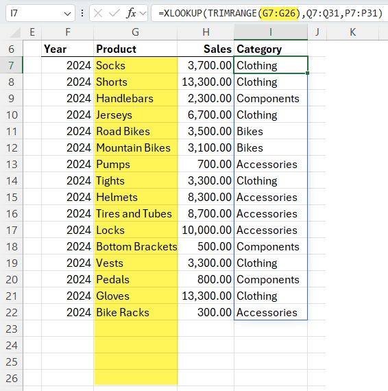
1. TRIMRANGE: The End of OFFSET Nightmares

Tired of writing complex OFFSET formulas for dynamic ranges? Enter the new TRIMRANGE function.

This function auto-detects the actual range of your data - trimming leading/trailing empty rows or columns.

Example – the formula below looks up the range G7:G26, but only returns results up to row 22 i.e. for the rows that contain data:

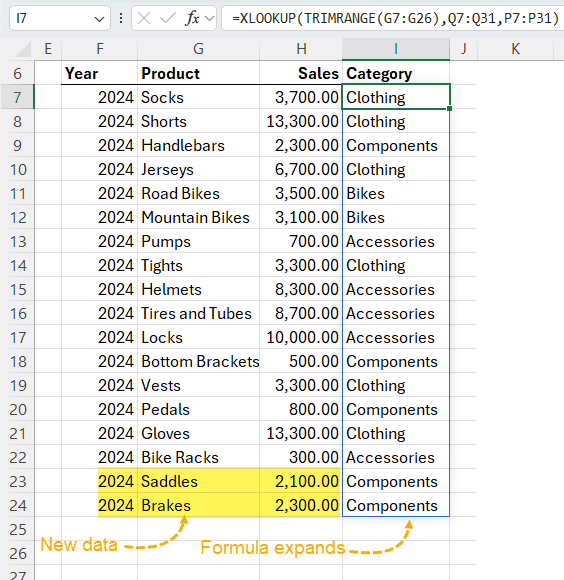
As you add more data to column G, the XLOOKUP will automatically expand to include it without having to edit the formula:

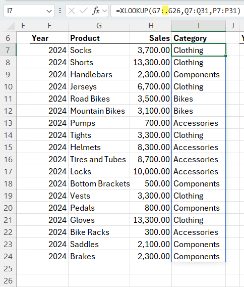
Tip: You can also use the Trim Ref Dot Operator for shorthand:

=XLOOKUP(G7:.G26,Q7:Q31,P7:P31)

The dot after the colon trims trailing blanks.

Placing a dot before the colon trims leading blanks or either side of the colon trims both leading and trailing blanks. e.g.:

=SUM(C.:.C)

Limitations: Not backward compatible with Excel 2024 and earlier.

Deep Dive Lesson: in the comprehensive TRIMRANGE and Trim Ref Dot Operator lesson I cover more uses for TRIMRANGE and the trim ref dot operator and why you’d use it instead of Table Structured References.

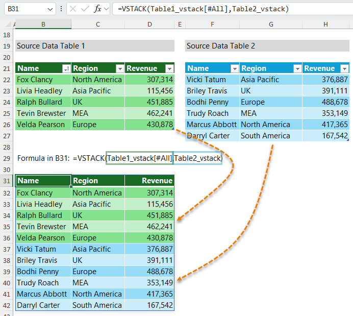
2. VSTACK: Stack Tables Without Power Query

Still got data spread across multiple sheets or tables? While Power Query is great at consolidating this data, sometimes you need something faster that updates automatically.

Example:

VSTACK(Table1_vstack[#All], Table2_vstack)

Tip: You can even use 3D referencing i.e. multiple sheets to consolidate data spread throughout your workbook:

=VSTACK('2023:2025'!A2:D6)

Limitations: VSTACK doesn't preserve formatting - apply it manually before or after stacking, or automate with conditional formatting. Requires Microsoft 365 or Excel 2024 or later.

Deep Dive Lesson: in this comprehensive VSTACK lesson, I also cover error handling, zero rows, and the sibling function, HSTACK.

3. BYROW: Row-Wise Formulas Just Got Easier

Stop dragging formulas down!

BYROW lets you write one formula and automatically apply it to every row in a range.

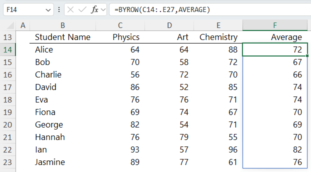
Example – find each student’s average student score:

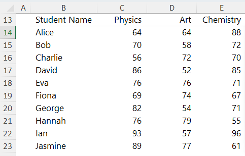
We can use this single BYROW formula:

=BYROW(C14:E23, AVERAGE)

Tip: Pair it with TRIMRANGE to future-proof it so it automatically expands as new data is added:

=BYROW(C14:.E30, AVERAGE)

Limitations: causes #SPILL! errors in Excel Tables, but this is where TRIMRANGE and the Trim Ref Dot operator save the day. Requires Microsoft 365 or Excel 2024 or later.

Deep Dive Lesson: BYROW has a sibling function for columns called BYCOL covered in the comprehensive BYROW & BYCOL lesson.

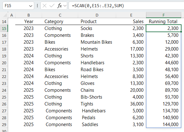
4. SCAN: Effortless Running Totals

Accountants rejoice – the SCAN function makes running totals a breeze.

Example – return the running total for the values in cells E15:E30:

=SCAN(0, E15:.E30, SUM)

Tip: team it up with the trim ref dot operator and it automatically adjusts as you add new rows - perfect for monthly transaction logs.

Limitations: causes #SPILL! errors in Excel Tables. Use TRIMRANGE or the Trim Ref Dot operator for dynamic ranges. Requires Microsoft 365 or Excel 2024 or later.

5. FILTER: The Swiss Army Knife of Lookup Functions

If you only learn one function from this post, let it be FILTER. It’s like VLOOKUP on steroids.

Use it to create dynamic reports, drop-down selectors, and more.

Example: Extract the data for the Sales department from the table below:

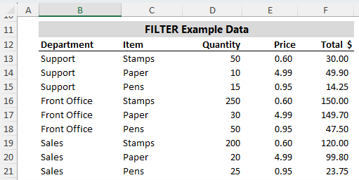
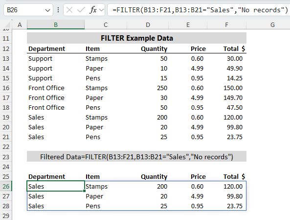
The FILTER formula below takes the table range, tests where the department = Sales, and if no records are found, it’ll return the text “No Records”:

=FILTER(B11:F19, B11:B19="Sales", "No Records")

You can see the results in rows 26:28 below:

FILTER is my favourite function - and this blog barely scratches the surface.

Limitations: Requires Microsoft 365 or Excel 2024 or later.

Deep Dive Lesson: in the comprehensive FILTER function lesson see how you can filter using multiple criteria, handle OR criteria, and extract non-contiguous columns. You can also link FILTER to data validation lists for interactive reports.

6. GROUPBY: PivotTables with Auto-Update Superpowers

PivotTables are great - but they don’t auto-refresh with new data. GROUPBY solves that.

Example:

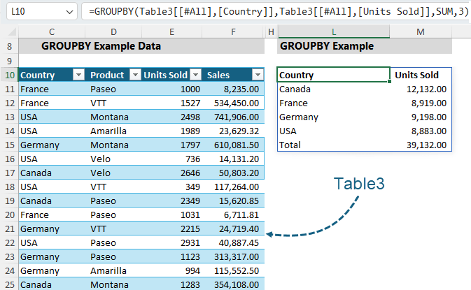
=GROUPBY(Table3[Country], Table3[Units Sold], SUM, 3)

Returns a summary of the sales in Table3 by country and includes a grand total:

Deep Dive Lesson: GROUPBY also supports:

• Non-contiguous columns
• Multiple value columns
• Sorting & filtering options

Check out the GROUPBY lesson to get up to speed.

Limitations: GROUPBY doesn't apply formatting – use conditional formatting to detect headers and totals and automatically apply formatting that adjusts with your data. Requires Microsoft 365 or Excel 2024 or later.

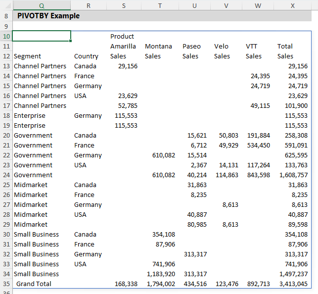
7. PIVOTBY: PivotTables with Rows and Columns via Formula

PIVOTBY is the sibling to GROUPBY, and it gives you full pivot control in a formula. Take this data in Table2:

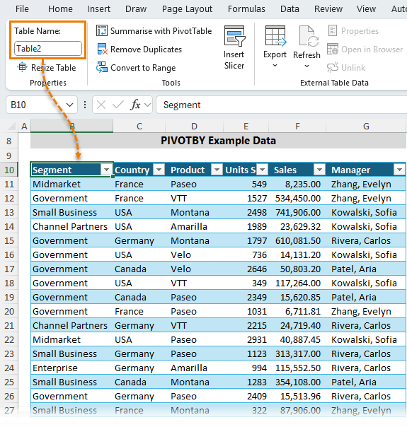
With this formula:

Limitations: PIVOTBY doesn't apply formatting – use conditional formatting to detect headers and totals and automatically apply formatting that adjusts with your data. Not compatible with Excel 2024 or earlier.

Deep Dive: you can also include subtotals, and link to slicers for interactivity which I cover in the comprehensive PIVOTBY lesson.

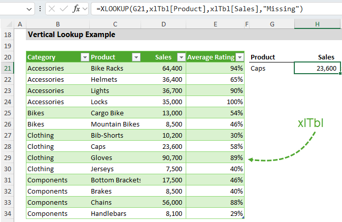
8. XLOOKUP: Finally, a VLOOKUP That Just Works

Say goodbye to VLOOKUP, HLOOKUP and nested INDEX/MATCH formulas.

Vertical Lookup:

=XLOOKUP(G21, xlTbl[Product], xlTbl[Sales], "Missing")

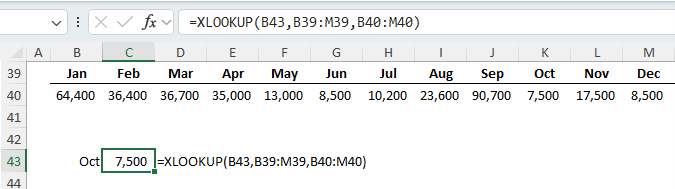
Horizontal Lookup:

XLOOKUP isn’t limited to looking up vertical arrays, it can lookup horizontally too:

Limitations: Requires Microsoft 365 or Excel 2021 or later.

Deep Dive: in the comprehensive XLOOKUP lesson you can also see how to:

• Return multiple columns/rows
• Return the last or first match
• Return an approximate match
• Two-way lookups
• Handle errors

9. LET: Reusable Variables for Clean, Fast Formulas

LET makes formulas readable and efficient by enabling you to name variables which are later used in the formula:

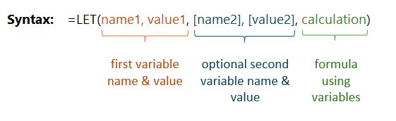
Easy example:

=LET(x, 5, y, 10, x + y)

Useful in more complex formulas in reducing repetitive calculations. In the formula below, the current year sales (SalesCY) are calculated once:

Whereas in a regular IF formula, the sum formula for SalesCY: SUM(C29:C38) would be calculated twice: once in the logical test and again in the value_if_true or value_if_false arguments.

When you have thousands of these formulas in your spreadsheets, the efficiency gains can be substantial.

Limitations: Requires Microsoft 365 or Excel 2021 or later.

Deep Dive: see the comprehensive LET lesson for more advanced uses, as well as tips on debugging.

10. SEQUENCE + DATE: Auto-Generate Date Lists

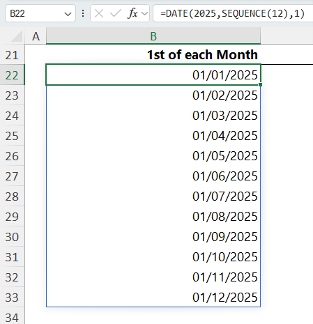
Use the SEQUENCE function with DATE to create a list of rolling date ranges instantly. Here’s how to get the 1st of each month:

=DATE(2025, SEQUENCE(12), 1)

It spills a list of dates for the first of each month for 2025:

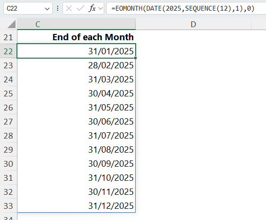
Or team it with the EOMONTH function to get the end of each month:

=EOMONTH(DATE(2025, SEQUENCE(12), 1), 0)

Tip: the DATE function can even handle overflow months which means you can make lists for 2 or more years by entering as many months as required in the SEQUENCE function. The example below returns 2 years of month end dates:

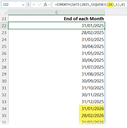
This works because Excel allows the month argument in DATE to go beyond 12 and it automatically rolls over to the correct month and year. So:

=DATE(2025, 13, 1) returns Jan 1st, 2026

And so on.

Limitations: Requires Microsoft 365 or Excel 2021 or later.

Bonus: Want to Master These and More?

If you’re enjoying these tips, you’ll love our Excel Expert Course. It’s self-paced, packed with real-world examples, and includes direct support from Microsoft MVP, Mynda Treacy, plus a certificate to boost your CV.

 Explore the Excel Expert course here