Handling messy data is a common challenge for anyone working with Excel. Tasks such as splitting columns, merging tables with VLOOKUP or XLOOKUP, unpivoting, transposing data, and removing duplicates can be tedious, especially if they need to be repeated regularly.
Imagine cutting your data cleanup time in half!
That's what Emmanuelle did with Power Query to gather and clean their data:

With Power Query you can save up to 95% of the time you'd normally spend on repetitive tasks, and the best part is with Power Query you don't need to know how to write code or even record a macro.
It's all point and click easy!
Here 6 essential Power Query data cleaning tips and tricks to make your life a whole lot easier.
Table of Contents
Watch the Video

Download Workbook
Enter your email address below to download the sample workbook.

1. Splitting Rows
Scenario: You have a table of everyone's favourite movies listed in a single cell, separated by commas:

And you want to make a list in a column:

- Load Data to Power Query:
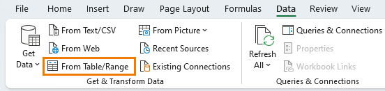
Tip: CTRL+T to format your data in an Excel table first.
- Split Column by Delimiter: On the Home tab, select "Split Column by Delimiter":
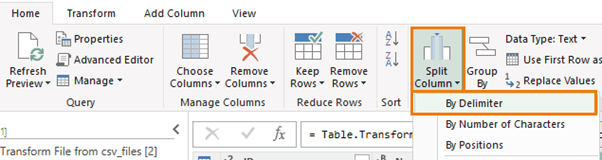
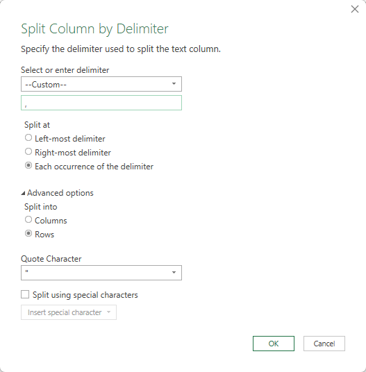
- Choose a custom delimiter and enter a comma followed by a space.
- Split at each occurrence of the delimiter.
- Under Advanced options, select "Split into rows"
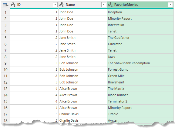
Now I have a list of the movies in a single column:
2. Grouping Data
Scenario: Some of the movies in the previous example are duplicated. To identify which movies are most popular, I can group and count them.
- Group Movies: Group the FavoriteMovies column and add a count to see which movies are most popular:
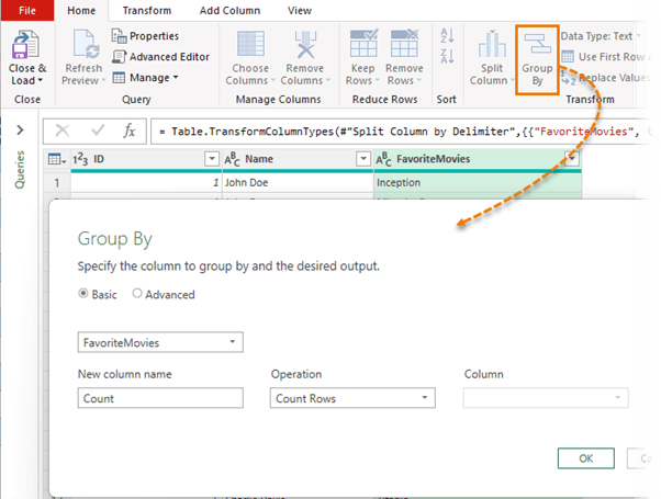
- Sort Data: Sort the list in descending order based on the count and then by movie name:

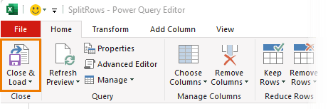
- Close & Load: Load your cleaned data back to Excel:
By default, it will load the table of data on a new sheet in the workbook.

3. Splitting by Digits
Scenario: You need to separate alpha and numeric characters in product codes, which vary in length and number of alpha vs numeric characters.
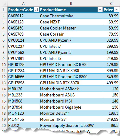
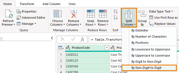
- Load Data to Power Query: Select the ProductCode column.
- Split Column by Non-Digit to Digit: On the Home tab, choose "Split Column by Non-Digit to Digit."
Now you will have two separate columns for the ProductCode:
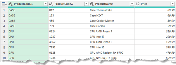
- Rename Columns: Double-click to rename the columns (e.g., ProductCodeAlpha and ProductCodeNumeric).
- Close & Load: Load the updated data back to your file.
4. Importing Data
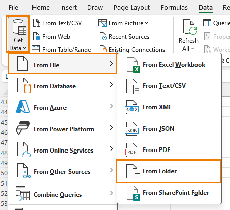
Scenario: You need to import and consolidate data from multiple CSV files into one table for a report.

- Get Data from Folder: Use "Get Data > From File > From Folder" to browse the folder containing your CSV files.
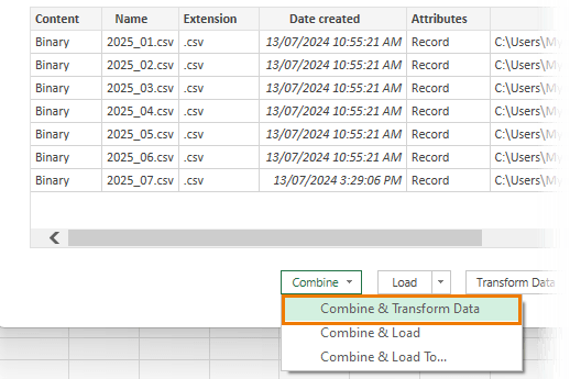
- Combine & Transform: Select "Combine and Transform" to clean data before loading it.
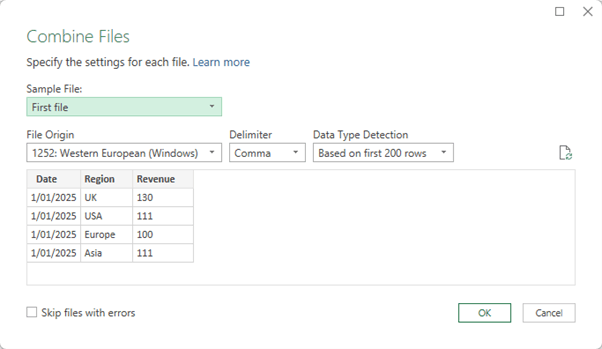
At the "Combine Files" dialog box, specify the file origin and delimiter if needed.
- Power Query Editor: View the queries created to combine the files and make additional adjustments if necessary (e.g., deleting columns, adding calculations).
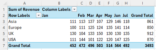
- Close & Load to PivotTable: Load the data to a PivotTable for easy summarization.
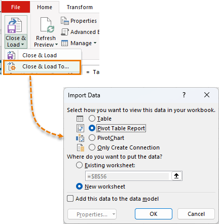
- Build Report: Select the fields you want to display in your report:
- Add New Data: add next month's file to the folder.

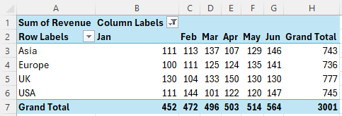
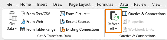
- Refresh All: Update your report with new data by clicking the Refresh All button on the Data tab:
And your report now includes the new data for July:
Tip: you can have multiple PivotTables and charts all linked to the query data and they will all update on clicking Refresh All.
5. Compare Lists/Tables
Scenario: Compare two employee lists to identify which employees are on both lists.
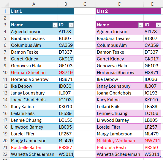
Note: I've highlighted names in red that are only on one list for illustrative purposes.
- Load Tables to Power Query: Format your data as Excel tables and load them.
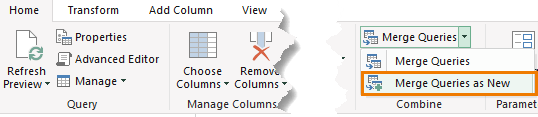
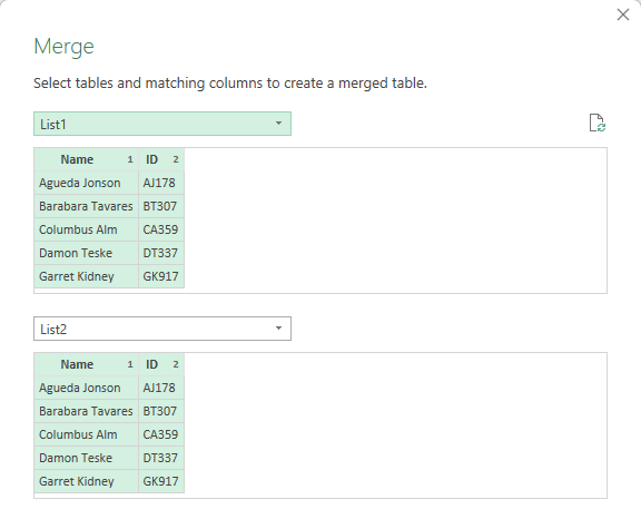
- Merge Tables: Use "Merge Queries" as a new table:
- Select Columns to Compare: Left click on the columns to match one by one. Hold CTRL to select more than one column in each table.
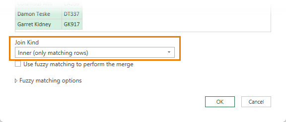
- Choose Join Kind: Select "Inner" join to find matching rows:
- Clean Up Data: Delete unnecessary columns and rename the query (e.g., CompareLists).
- Experiment with Joins: Try different join types. For example, Full Outer to see all rows from both tables.
6. Unpivoting Data
Scenario: You have pivoted sales data with multiple columns containing the same type of data, e.g. sales values:
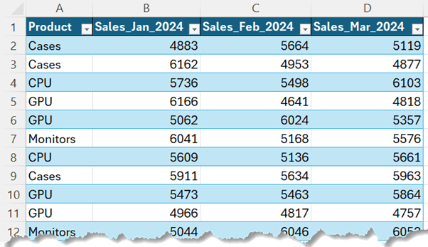
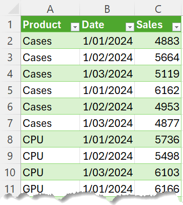
And you need to convert it into a tabular format:
- Load Data to Power Query: Load your pivoted data.
- Unpivot Columns: Right-click on the Product column and select "Unpivot Other Columns."
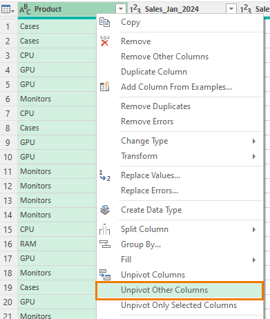
This will ensure when new months are added to the data, they too are automatically unpivoted on refreshing the query.
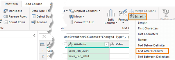
- Clean-up Date Column: Extract text after delimiters:
And replace underscores with slashes to format dates correctly:
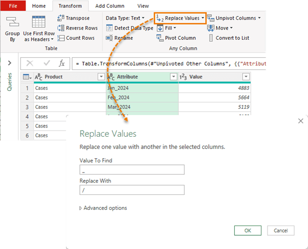
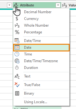
- Change the data type to date: click on the ABC drop down to the left of the column header and choose 'Date':
- Rename Columns: Double click Attribute and Value column headers to rename them to Date and Sales.
- Close & Load: Load the cleaned data back to Excel for further analysis.
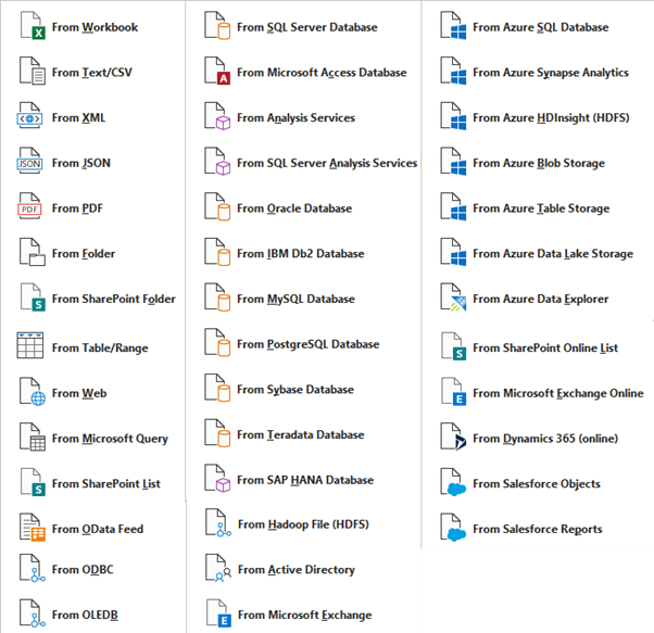
Automating Data Import
Power Query is not just for cleaning data; it also automates data imports from various sources (see image below) such as Excel files, databases, web pages, PDFs, and images. This automation cuts down on repetitive data gathering tasks, allowing you to focus on analysis and reporting.
Next Steps
As you can see, automating the gathering and cleaning of data with Power Query is a game changer. If you're serious about taking your Excel skills to the next level and improving productivity, Power Query is the way to go.
But don't take my word for it. Here's a survey I posted on YouTube a few weeks ago:
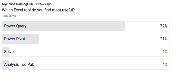
And here are some of the comments left on the survey page:

If you'd like to get your Power Query skills up to speed, please consider my comprehensive Power Query course, I cover everything from the basics to advanced techniques.
Plus, I provide support both during the tutorials and when you're implementing the techniques in your own work.


Awesome post! I have this flagged in my inbox to come back to reference, since it is so great. With comparing lists, I love using left anti join to produce items that are not in the “other” list, as well!
Great to hear, Matt! Thank you.