I know you’re probably thinking that everyone knows how to use the SUM function, but I’m willing to bet that most people don’t know all the shortcuts and tricks I’m about to show you. These are SUM function tricks you can use every day, and some also apply to all Excel functions.
Watch the Video

Download Workbook
Enter your email address below to download the sample workbook.

Excel SUM Function Tricks
Trick 1: AutoSum
AutoSum detects the range you want to sum by looking for rows/columns adjacent to the cell you have selected that contain numbers. You’ll find it on the home tab:
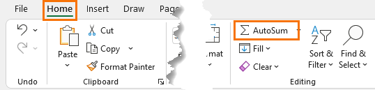
However, I find the keyboard shortcut ALT+= easier to use.
Tip: Select the whole table plus a blank row and column for the sum formulas and ALT+= to automatically enter the SUM formulas for each row and column:
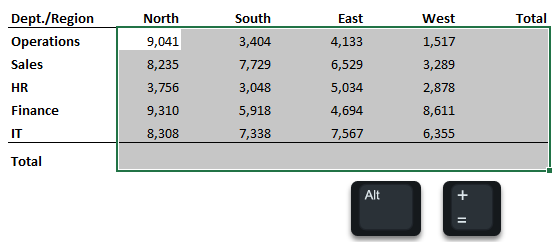
Bonus tip: you can select non-contiguous ranges and press ALT+= to insert multiple AutoSums – see video for demo.
Trick 2: CTRL shortcut for non-contiguous ranges
If you want to sum non-contiguous cells, hold the CTRL key while you select the cells with your mouse to have Excel automatically insert the comma separators for you. This works for other functions too.
Bonus tips not in the video from Bob Umlas - AutoSum Subtotals: To insert a Grand Total for a range of cells containing sub-totals, select the whole range including the cell you want your grand total in > ALT+=
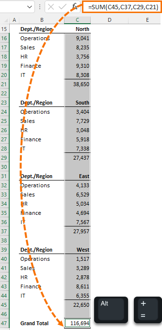
Or simply SUM the entire range and divide by 2 e.g. using the example data above in cell C47 enter this formula:
=SUM(C16:C45)/2
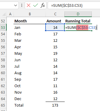
Trick 3: Running Total
To insert a running total reference the first cell in the range, then Absolute reference the first cell in the range before copying the formula down:
Trick 4: SHIFT for 3D ranges
Sum multiple contiguous sheets by selecting the cell on the first sheet and while holding the SHIFT key, select the last sheet in the range:
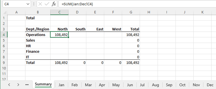
Caution: This will sum all sheets from Jan to Dec. If you drag another sheet inside this range, it will also be included in the sum.
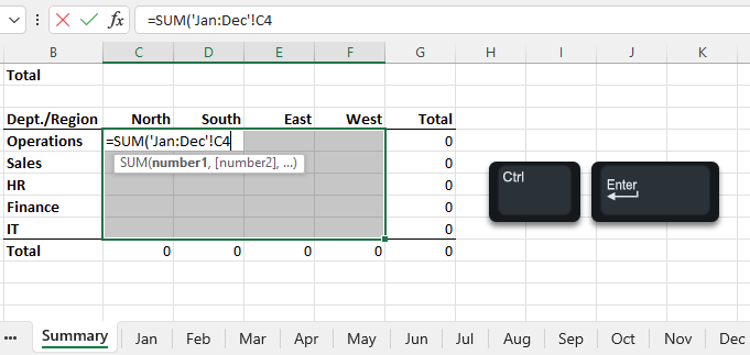
Trick 5: Insert multiple SUM formulas in one go with CTRL+ENTER
Select all the cells you want your SUM formulas in, then enter the first formula and CTRL+ENTER to complete the formula:
If you have a SUM tip or trick, please share it in the comments below.

It has been a long time since I used MC excel. I’ve been retired many years and I haven’t had the need to do formulas for bookkeeping and other documents. I am trying to make an Estate checkbook for my son, that I need to keep an record of incoming monetary amounts and Debits going out and balance. I have tried several formulas that I remember but its not working for me. Is there any temp plate or an formula that you could email me?
Thank you for your help.
Jan Smith
Hi Jan,
I don’t have a template as such, but you might find these tutorials on running totals helpful:
Running Total Formula – not Excel Tables
Running Total Formula – for Excel Tables
You might also find this tutorial on my personal finance dashboard relevant for the reporting.
Mynda
Hi
Please assist me with a countifs formulae
STATUS No of Quotes Value of Quotes
Accepted 4 0
Pending 3 0
ReQuote 1 0
Cancelled 2 0
Total Quotes Issued 10
QUOTE NO DATE CUSTOMER VALUE STATUS
160285 2022-06-10 Unilever R 2 500.00 Accepted
160286 2022-06-11 Sab R 1 680.00 Accepted
160287 2022-06-12 Colgate R 1 120.00 Pending
160288 2022-06-14 Cipla R 3 600.00 ReQuote
160289 2022-06-20 Unilever R 850.00 Cancelled
160290 2022-06-21 Cipla R 925.00 Pending
160291 2022-06-22 Sab R 865.00 Cancelled
160292 2022-06-24 Unilever R 340.00 Accepted
160293 2022-06-24 Unilever R 2 800.00 Pending
160294 2022-06-25 Unilever R 1 468.00 Accepted
Hi Johnny,
Please see this COUNTIFS tutorial. If you get stuck please post your question on our Excel forum where you can also upload a sample file and we can help you further.
This is great!!
Can I access the workbook to practice?
Glad you liked it, Brian. Please see the link to the workbook in the post above which I’ve just added.
Everything else
I will definitely add ALT+= to my list, thanks!
May not be as fast as keyboard shortcuts, but the Quick Analysis toolbar can add not only SUM, but AVERAGE, COUNT, % TOTAL and RUNNING TOTAL to rows or columns. Also, if you are just interested in getting an idea of those numbers without actually adding the formulas, it gives you a preview of the result. Just highlight the range with your numbers and click the Quick Analysis icon that pops up on the lower right of your selection.
Great post as usual, thanks again!
Great to hear, Ben! Thanks for sharing your tips too.
Thanks so much Mynda for another great & clear how to!
Here are some other useful tricks:
Example 1: Summarize absolute values
{=SUM(ABS(A1:A4))} – this is an array formula; the curly braces don’t need to be manually typed, as they are automatically inserted by using CTRL+SHIFT+ENTER
Example 2: Summarize the last 10 values in a list (cell A1 is header)
=SUM(OFFSET(A1,ROWS($A$2:$A$25),0,-10))
Example 3: Summarize intersection of ranges
=SUM(B2:F6 D4:H8)
Example 4: Summarize only the integer part of the numbers from a list
{=SUM(TRUNC(A1:A4))} – this is an array formula (see previous note)
Example 5: Summarize Top 5 numbers from a list
{=SUM(LARGE(A1:A10,{1,2,3,4,5}))} – this is an array formula (see previous note)
or
{=SUM(LARGE(A1:A10,ROW(INDIRECT(“1:5”))))} – this is an array formula (see previous note)
Example 6: Summarize the digits of a number
{=SUM(1*MID(A1,ROW(INDIRECT(“1:”&LEN(A1))),1))} – this is an array formula (see previous note)
Thanks so much for sharing, Andrei!