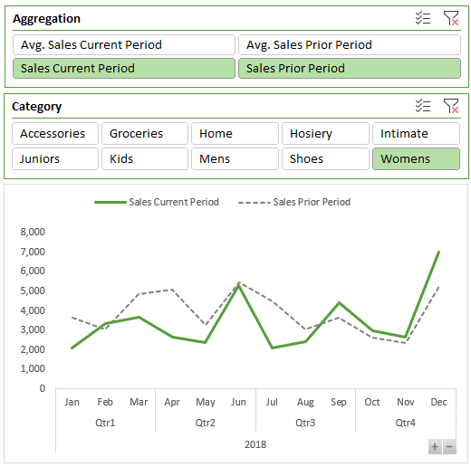
With disconnected tables in Power Pivot* we can change PivotChart aggregation methods using Excel Slicers. It allows us to create Pivot Charts where the user can select different views of the data like so:
It’s handy if you have limited space in your report or dashboard, as it allows you fit two charts into one.
*Click here to see if your version of Excel supports Power Pivot.
This post assumes you are familiar with Power Pivot (aka the Data Model), can load data to the model and create relationships. If you’d like to learn Power Pivot, please consider my Power Pivot course.
Power Pivot Model Structure
The model contains a table for the facts i.e. the transaction data, called ‘Sales’. There’s also a Calendar table because the sales transactions are not on consecutive dates, which are required for the prior period measures below. And finally a table for the aggregation type.
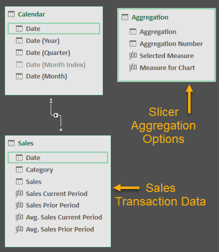
Tip: Notice that the Aggregation table is not connected to any other tables.
Power Pivot Measures
There are four measures that aggregate the sales values for the current period and prior period:
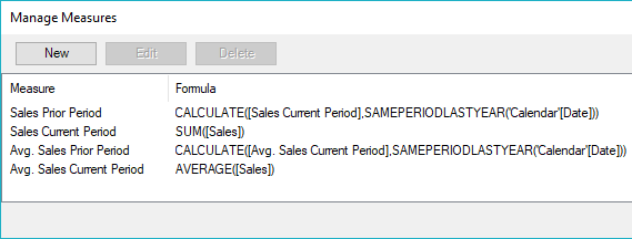
You can create more measures if required.
Disconnected Table
The trick to this is creating a disconnected table that we use to feed the Slicer. It’s just a Table in Excel that lists the measures/aggregations that I want the user to choose from, which I’ve loaded into the Power Pivot model.
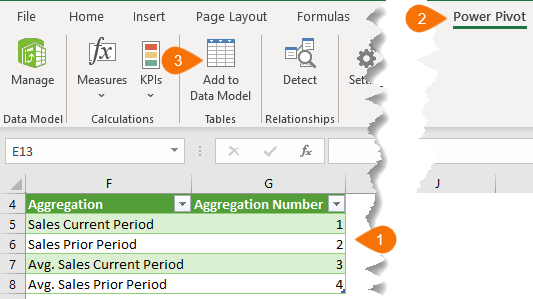
Remember, this table doesn’t get connected to any other tables in the model.
Next you need to set up a measure for this table that detects the aggregation number selected in the Slicer. Mine is called ‘Selected Measure’:
=MIN(Aggregation[Aggregation Number])
Then create another measure with the SWITCH function that takes the ‘Selected Measure’ value and returns the corresponding measure. Mine is called ‘Measure for Chart’:
=SWITCH(
[Selected Measure],
1, [Sales Current Period],
2, [Sales Prior Period],
3, [Avg. Sales Current Period],
4, [Avg. Sales Prior Period]
)
PivotTable
The PivotTable uses the field; ‘Aggregation’ in the column labels and the field; ‘Measure for Chart’ in the Values area. I’ve used dates in my row labels because my Sales table prior period measures require them.
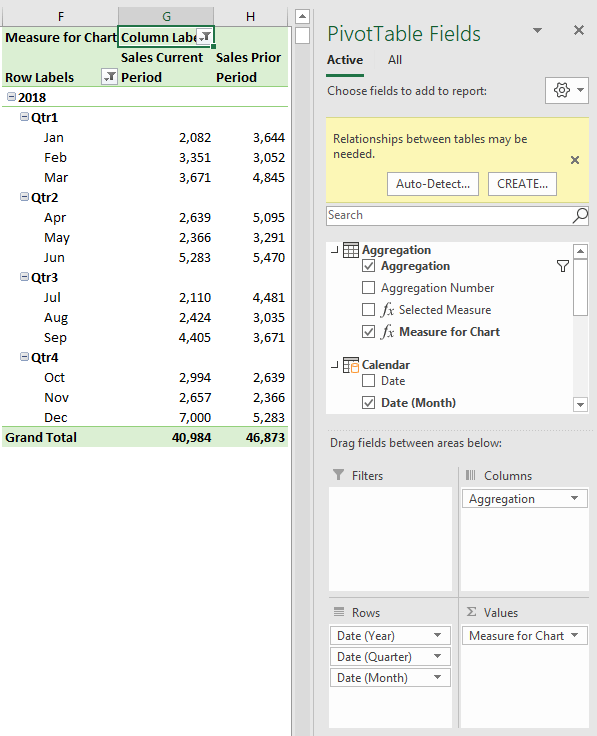
Note: You can ignore the Relationship warning in the field list that appears when you add ‘Aggregation’ and ‘Measure for Chart’ to the PivotTable.
PivotChart
And finally, insert your Slicer for the Aggregation type (and any others you want), and the Pivot Chart:
Download Workbook
Enter your email address below to download the sample workbook.
Thanks
Thanks to Erik Svensen for sharing this idea.
Hello,
This is a dream. I humbly bow before you.
Seriously this is amazing!
astier
🙂 glad you can make use of it!
Hi Mynda – I have just emailed the downloaded file to you along with sample screen shots of what I was experiencing. Frans
Thanks, Frans.
It’s just that the line has lost its formatting. If you go to the PivotTable format tab and in the ‘Current Selection’ group choose the series from the drop down you can then add some colour back to the line (outline).
You’ll have to do this for each series that’s missing the data, but once you’ve set them all up they’ll stick.
Mynda
Hi Mynda – fyi – When I opened the sample file and changed aggregation selections the chart lost the line colour – i.e. the plot area appeared blank (this occurred in Office 365 Business – Excel Version 1903 and also in MS Office Professional Plus 2016). Kind regards, Frans
Hi Frans,
That’s strange. Can you please send the file to me: website at myonlinetraininghub.com
Mynda
Thanks for the mention 😉
🙂 of course.